Economics of Education Review 20 (2001) 165–180
www.elsevier.com/locate/econedurev
Educational attainment and the gender wage gap: evidence
from the 1986 and 1991 Canadian censuses
Pamela Christie
a, Michael Shannon
b,*aIndian Affairs and Northern Development Canada, 10 Wellington St., Hull, PQ, Canada bDepartment of Economics, Lakehead University, Thunder Bay, Ontario, Canada
Received 20 August 1998; accepted 20 July 1999
Abstract
The paper takes advantage of the detailed information on educational attainment and field of study provided in the Canadian Census to examine gender differences in educational attainment and the effect of these differences on the gender earnings gap for full-time, full-year workers in Canada. Gender differences in field of study of post-secondary graduates are found to be an important contributor to the gap. This is an important finding given the lack of such data in most studies of the gender gap. Gender differences in educational attainment account for virtually none of the gender gap in earnings in 1985 and 1990 — a result also found in earlier studies using less detailed attainment data. However, projections suggest that although gender differences in attainment explain little of the gap in these years, the continuing improvement in women’s educational attainment relative to men has helped shrink the gap in the past and will likely continue to do so.2001 Elsevier Science Ltd. All rights reserved.
JEL classification:I2; J7; J3
Keywords:Education; Gender; Wages; Canada
1. Introduction
Human capital theory suggests that educational attain-ment will be an important determinant of labour earn-ings. Consequently, differences by gender in educational attainment are a candidate for explaining the male-female earnings gap. Canadian studies of the gender wage gap have attempted to measure the impact of edu-cation by including eduedu-cational variables in their analy-ses. A simple years of education regressor or a set of educational attainment dummies are typical.1The Census
* Corresponding author. Tel.:+1-807-343-8382.
E-mail address: [email protected] (M. Shannon).
1 Baker, Benjamin, Desaulniers and Grant (1995), for example, use a years of education variable in their analysis of the gender gap using 1971, 1981 and 1986 census data. Miller (1987) also uses a years of education measure. Studies relying
0272-7757/01/$ - see front matter2001 Elsevier Science Ltd. All rights reserved. PII: S 0 2 7 2 - 7 7 5 7 ( 9 9 ) 0 0 0 5 8 - 8
provides more information on educational attainment than other Canadian microdata surveys. Furthermore, the most recent censuses have provided information on field of study for post-secondary graduates. This paper uses this superior data source to further investigate the impact of education on the gender gap in Canada.
The paper begins with a description of the educational data available from the 1986 and 1991 censuses. Differ-ences in educational attainment and field of study by gender are then described and variation by year and age grouping is used to infer how these differences have changed over time. Data on earnings by education level are presented in Section 3 and some simple calculations of the importance of education to the gender wage gap
are made. Section 4 presents econometric estimates of male and female earnings equations and assesses the importance of disaggregated education data in explaining variation in earnings. The log-earnings gap is decom-posed into residual and explained parts and the share of education in explaining the gap is calculated in Section 5. Section 6 compares the results to those of earlier stud-ies.
2. Data
The data used in this paper are from the public use subsamples of the 1986 and 1991 Canadian censuses.2
The earnings data apply to the years 1985 and 1990. The focus is on the sample of wage and salary earners who worked full-time and full-year3and who were aged 25–
64. From our perspective, the availability of detailed educational attainment information is the principal advantage of using the Census to study the gender wage gap while information on field of study dictates the choice of census years 1986 and 1991. Other important advantages of census data include the large sample size, and consequent increased statistical reliability of the results, and the detailed data on personal characteristics it contains. The main disadvantage of using the Census to study earnings differentials is its lack of information on job characteristics other than industry and occupation. A brief overview of the Canadian education system which the education variables describe is provided in the Appendix A. The public use version of the Census microdata file contains seven education variables in 1986 and ten in 1991. All but one of the variables measures the level of educational attainment. The most complete of these is “Highest Level of Schooling” which con-tained 11 categories in 1986 and 14 in 1991.4 The
remaining educational variable in each data set reports the field of study for those with post-secondary qualifi-cations.
This array of education variables is generous in com-parison to those available in other Canadian microdata surveys. For example, the public use version of the much used Labour Market Activity Survey (1986–87, 1988– 90) contains one educational attainment variable with seven possible values. Educational detail in the Survey of Consumer Finances, Canada’s main source of annual
2 The subsample is a 2% (1986) or 3% (1991) sample of Canadian households.
3 The definition of full-time/full-year used is: worked at least 30 hours/week for 49 to 52 weeks of the year. Focus on this subsample ignores any effect education may have on earnings through its effects on hours and weeks of work.
4 The other attainment variables provide details on years of schooling by level or information on degree attained.
income data, is similarly limited. Furthermore, earlier versions of the census lack data on field of study.5
The main education variable used in the analysis below combines the “Highest Level of Schooling” and the “Highest Degree, Certificate, Diploma Attained” variables. The resulting composite variable has nineteen classifications which are reported in Table 1 along with the shares of the samples of full-time, full-year workers who fall into each of these categories in the 1991 and 1986 censuses.
In the 1991 census, the largest shares of men and women are found in the four categories: grades 9–13, high school graduate, non-university certificate and Bachelor’s degree. Together these levels accounted for about 54% of the male sample and 62% of the female sample. Men are more likely than women to have less than high school education (23% vs. 20% in 1991) while women are more likely to be high school graduates by nearly the same margin. The male share was nearly twice the female share across the three trades categories in 1991. Women were more likely to have a trade, non-university certificate or diploma than men. There were near equal shares of men and women with Bachelors degrees while the male shares were higher for graduate level degrees.
The pattern of educational attainment was similar in the 1986 Census. The most notable changes between 1986 and 1991 were the decline in the share of those with the lowest levels of education, the rise in the share with high school and the rise in the shares with univer-sity degrees.
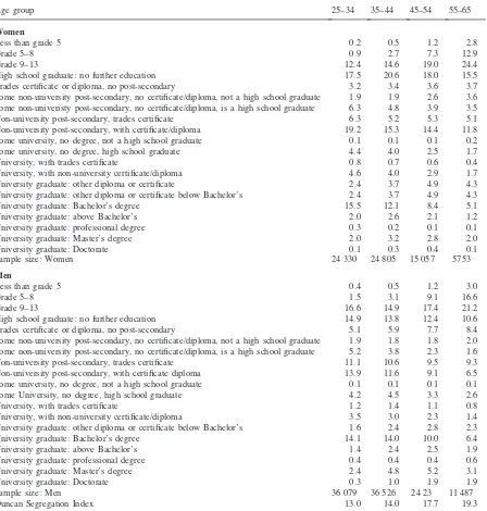
The changes in educational attainment over time become more evident in Table 2 which reports 1991 edu-cational attainment by age group. The shares with the lowest levels of education are much larger for the older age groups. There are correspondingly larger shares of university educated workers and workers with post-sec-ondary certificates among the younger groups. It is also apparent that educational attainment of women has been improving relative to men. The share of younger women with university degrees is much higher than for older women and has actually overtaken the share of young men with degrees. Women’s educational attainment has also improved relative to men at the lower end. The share of women with less than high school has fallen more sharply across age groups for women — for 55–64 year-olds this share was roughly 40% for both sexes but had fallen to 18.5% for men and 13.5% for women in the 25–34 age group.
The figures in Tables 1 and 2 are for a sample of
167
P.
Christie,
M.
Shannon
/
Economics
of
Education
Review
20
(2001)
165–180
Table 1
Educational attainment of full-time workers, full-year workers
Acronym Definition 1986 census 1991 census
Women Men Women Men
Share (%) number Share (%) number Share (%) number Share (%) number
LT5* Less than grade 5 1.2 411 1.2 734 0.8 527 0.9 927
GR58 Grade 5–8 6.0 2101 8.4 5076 3.9 2729 5.4 5814
GR913 Grade 9–13 19.8 6907 19.6 11850 15.6 10919 16.7 18087
HS High school graduate: no further education 16.6 5780 11.8 7107 18.6 12989 13.5 14638 TRD1 Trades certificate or diploma: no post-secondary 2.4 838 4.8 2918 3.4 2362 6.3 6846 SPNHS Some non-university post-secondary, no 5.0 1744 4.1 2472 5.0 3489 3.7 3999
certificate/diploma, not a high school graduate
SPHS Some non-university post-secondary, no 5.8 2025 9.5 5726 5.6 3899 10.4 11255 certificate/diploma, is a high school graduate
TRD2 Non-university post-secondary, trades certificate 14.4 5000 9.6 5775 16.2 11329 11.3 12216 PSCD Non-university post-secondary, with 14.4 5000 9.6 5775 16.2 11329 11.3 12216
certificate/diploma
SUNHS Some university, no degree, not a high school 0.8 268 0.8 494 0.1 74 0.1 117 graduate
SUHS Some University, no degree, high school graduate 2.8 967 3.4 2022 3.6 2542 3.9 4228 UTRD3 University, with trades certificate 0.7 256 1.1 690 0.7 479 1.2 1310 UNUC University, with non-university certificate/diploma 3.5 1216 2.7 1624 3.8 2625 2.8 3073 ULTB University graduate: other diploma or certificate 3.5 1213 2.3 1376 3.5 2482 2.2 2397
below Bachelor’s
BACH University graduate: Bachelor’s degree 10.6 3684 11.3 6787 11.9 8332 12.3 13375 BACH+ University graduate: above Bachelor’s 1.8 624 1.8 1058 2.2 1512 2.0 2199 UPROF University graduate: professional degree 0.2 59 0.3 194 0.2 135 0.4 463 MASTER University graduate: Master’s degree 2.1 732 3.7 2231 2.6 1815 3.9 4221 DOCT University graduate: Doctorate 0.3 119 1.2 699 0.3 186 1.0 1123
Total sample 34 831 60 306 69 945 108 323
Table 2
Educational attainment by age and sex (per cent), 1991 census
Age group 25–34 35–44 45–54 55–65
Women
Less than grade 5 0.2 0.5 1.2 2.8
Grade 5–8 0.9 2.7 7.3 12.9
Grade 9–13 12.4 14.6 19.0 24.4
High school graduate: no further education 17.5 20.6 18.0 15.5
Trades certificate or diploma, no post-secondary 3.2 3.4 3.6 3.7
Some non-university post-secondary, no certificate/diploma, not a high school graduate 1.9 1.9 2.6 3.6 Some non-univeristy post-secondary, no certificate/diploma, is a high school graduate 6.3 4.8 3.9 3.5
Non-university post-secondary, trades certificate 6.3 5.2 5.3 5.1
Non-university post-secondary, with certificate/diploma 19.2 15.3 14.4 11.8
Some university, no degree, not a high school graduate 0.1 0.1 0.1 0.2
Some university, no degree, high school graduate 4.4 4.0 2.5 1.7
University, with trades certificate 0.8 0.7 0.6 0.4
University, with non-university certificate/diploma 4.6 4.0 2.9 1.7
University graduate: other diploma or certificate 2.4 3.7 4.9 4.3
University graduate: other diploma or certificate below Bachelor’s 2.4 3.7 4.9 4.3
University graduate: Bachelor’s degree 15.5 12.1 8.4 5.1
University graduate: above Bachelor’s 2.0 2.6 2.1 1.2
University graduate: professional degree 0.3 0.2 0.1 0.1
University graduate: Master’s degree 2.0 3.2 2.8 2.0
University graduate: Doctorate 0.1 0.3 0.4 0.1
Sample size: Women 24 330 24 805 15 057 5753
Men
Less than grade 5 0.4 0.5 1.2 3.0
Grade 5–8 1.5 3.1 9.1 16.6
Grade 9–13 16.6 14.9 17.4 21.2
High school graduate: no further education 14.9 13.8 12.4 10.6
Trades certificate or diploma, no post-secondary 5.1 5.9 7.7 8.4
Some non-university post-secondary, no certificate/diploma, not a high school graduate 1.9 1.8 1.8 2.0 Some non-university post-secondary, no certificate/diploma, is a high school graduate 5.2 3.8 2.3 1.6
Non-university post-secondary, trades certificate 11.1 10.6 9.5 9.3
Non-university post-secondary, with certificate diploma 13.9 11.6 9.1 6.5
Some university, no degree, not a high school graduate 0.1 0.1 0.1 0.1
Some University, no degree, high school graduate 4.2 4.5 3.3 2.6
University, with trades certificate 1.2 1.4 1.1 0.8
University, with non-university certificate/diploma 3.5 3.0 2.3 1.4
University graduate: other diploma or certificate below Bachelor’s 1.6 2.4 2.8 2.3
University graduate: Bachelor’s degree 14.1 14.0 10.0 6.4
University graduate: above Bachelor’s 1.4 2.4 2.5 1.9
University graduate: professional degree 0.4 0.4 0.4 0.6
University graduate: Master’s degree 2.4 4.8 5.2 3.1
University graduate: Doctorate 0.3 1.0 1.9 1.9
Sample size: Men 36 079 36 526 24 23 11 487
Duncan Segregation Index 13.0 14.0 17.7 19.3
time, full-year workers — a select group, especially for women. Educational attainment is lower for the general population.6 This partly reflects the larger numbers of
older workers and partly the increased likelihood that better educated workers will work.
6 The share of the general population age 25–64 with less than high school is 26% compared to 22% for the sample of full-time, full-year workers. The share with a Bachelors degree
Table 3 reports field of study of those with post-sec-ondary qualifications, a group which accounts for roughly half the sample. For women, the most common fields were secretarial science, business, education and nursing. These accounted for over 62% of qualifications
169
P. Christie, M. Shannon / Economics of Education Review 20 (2001) 165–180
Table 3
Field of study of post-secondary graduates
Acronym Field name 1986 census 1991 census
Women Men Women Men
Share number Share number Share number Share number
(%) (%) (%) (%)
Share of post-secondary graduates:
EDREC Education/recreation 15.1 2838 6.0 1733 15.9 5591 6.1 3564
ARTS Fine and applied arts 4.6 729 2.7 780 5.5 1948 2.7 1586
HUMAN Humanities 8.1 1270 5.9 1709 6.8 2377 4.8 2832
SOCSC Social sciences 8.9 1411 8.9 2580 9.2 3227 8.7 5066
BUS Business 13.6 2149 16.9 4913 15.6 5491 16.7 9756
SECR Secretarial 19.0 3003 1.2 356 16.7 5867 0.09 523
AGRBIO Agriculture/biology 3.8 606 4.3 1252 3.7 1286 4.3 2509
ENGIN Engineering/applied science 0.5 85 7.7 2230 0.7 259 7.6 4455
ENGTR Engineering/applied science 3.4 529 38.6 11 216 3.7 1312 39.9 23 350 (technology and trades)
NURS Nursing 15.0 2361 0.7 197 14.2 4979 0.6 364
HEALTH Health (not nursing) 5.3 839 2.1 615 5.5 1925 2.5 146
MATHPH Math/physics 0.2 36 0.2 63 0.2 70 0.2 121
Share with post-secondary qualification 45.3 15 766 48.2 29 078 50.3 35156 54.0 58 478 Duncan segregation index 48.7 47.4
in both the 1986 and 1991 Censuses. Engineering and applied science dominates for men accounting for nearly 40% of qualifications in both years.7Business was a
dis-tant second in terms of importance (16–17%). The most sizeable change in field of study between 1986 and 1991 was the fall in the share of women in secretarial science. A breakdown of field of study by age shows that field of study patterns have not been nearly as stable as a com-parison of 1986 and 1991 figures in Table 3 might sug-gest. Nursing and education/recreation account for 38% of qualifications of women aged 55–64 in 1991 but only 21% of 25–34 year old women (see Table 4). Business qualifications, social sciences, health (non-nursing) and engineering have become more common for young women. Engineering/applied science dominates for both older and younger men but has diminished slightly in importance. The biggest share increase for men between age groups has been the rise in those with social science qualifications.8
similar to those in Table 1.
7 This dominance reflects the concentration of non-univer-sity technical and trades qualifications in this group. Among male post-secondary graduates with non-university qualifi-cations, 62.5% have engineering/applied science as a field.
8 The patterns for those with university degrees are substan-tially different. For women, the most common fields were edu-cation, social sciences, humanities and business. Together these accounted for about 3/4 of degrees in 1991. Business was most common for men followed by engineering, social sciences, edu-cation and math/physics — together accounting for 80% of
The value of the Duncan segregation index is reported in the last row of Tables 1–4. The index shows the share of workers of one sex who would have to change attain-ment (or field) to equalize attainattain-ment (or field) shares across genders and so provides a simple summary meas-ure of gender differences in educational outcomes.9The
index equalled 14.0 for educational attainment in 1991 (19.3 for the oldest group and 13.0 for those aged 25– 34) and 12.8 in 1986. Index values were much higher for field of study (47.4 in 1991 and 48.7 in 1986). As
degrees. A breakdown of field of study by age at the university level reveals that business has been the fastest growing field for both genders. 17.5% of women and 25.4% of men aged 25– 34 had business degrees in 1991 compared to 4.5% and 14.6% respectively for those aged 55–64. A larger share of younger than older women have degrees in social sciences while the shares in education, the humanities and nursing have fallen. Younger men are more likely to have degrees in engineering, the humanities and education and more likely to be in math/physics or the social sciences. The trends in business degrees, engineering and nursing have resulted in some conver-gence in field shares between the sexes.
9 The index is calculated as: 1
2
O
N
i51 |Mi2Fi|
whereMiis the share of the male sample that is in categoryi,
Fiis the share of the female sample that is in categoryiandN
Table 4
Field of study by age and sex, 1991 census Age groups
25–34 35–44 45–54 55–64 Women
Education/recreation 11.3 17.1 22.6 17.2 Fine and applied arts 6.9 5.0 4.1 4.7
Humanities 6.2 7.4 6.7 7.0
Social sciences 11.1 9.1 6.7 5.4
Business 18.8 14.3 12.5 12.8
Secretarial 16.7 16.2 16.5 20.7
Agricultural/biology 4.2 3.4 3.0 3.7 Engineering/applied 1.1 0.7 0.3 0.3 science
Engineering/applied 4.9 3.5 2.4 1.9 science
(technology/trades)
Nursing 9.5 15.2 19.6 20.9
Health (not nursing) 6.4 5.5 4.0 3.7
Math/physics 2.8 2.4 1.5 1.6
All other 0.2 0.3 0.2 0.3
Number with post- 13 689 12 598 6831 2038 secondary: Women
Men
Education/recreation 3.6 6.9 9.0 5.5 Fine and applied arts 2.5 2.6 2.8 3.5
Humanities 3.8 5.1 5.6 5.9
Social sciences 9.0 9.7 7.8 5.6
Business 17.6 16.7 15.7 15.3
Secretarial 0.6 0.8 1.1 1.9
Agricultural/biology 4.5 4.3 4.0 4.3 Engineering/applied 7.3 7.6 7.7 8.8 science
Engineering/applied 42.4 38.3 38.3 41.5 science
(technology/trades)
Nursing 0.6 0.8 0.5 0.5
Health (not nursing) 2.5 2.3 2.6 3.4
Math/physics 5.5 4.9 4.8 3.5
All other 0.2 0.2 0.2 0.4
Number with post- 19 909 21 018 12 689 4862 secondary: Men
Duncan segregation 46.7 47.9 51.8 53.6 index
with educational attainment, the index for field of study was highest for older workers and lowest for those aged 25–34. Calculation of the segregation index for occu-pation and industry revealed substantial differences in the type of jobs held by men and women. In 1986 the index was 30.5 for occupation and 44.0 for industry. These figures had fallen to 29.1 and 41.9 respectively by 1991.
3. Role of education in determining wage differences
Tables 1–4 illustrate significant gender differences in the level of educational attainment and the field of study and often document substantial changes over time. What are the consequences of these findings for the gender gap in earnings? The economics literature suggests that more education is associated with higher wages due to its effect on skills or possibly because it reveals something about the person’s innate abilities. This prediction has been verified by the vast majority of empirical studies. The field of study chosen gives access to different opportunities and labour markets and consequently it too will influence the level of earnings obtained.
A first impression of the importance of educational differences to the earnings gap can be obtained by look-ing at average wage and salary earnlook-ings figures by edu-cational attainment and field of study. Table 5 reports average annual earnings and the female–male average earnings ratio by level of educational attainment. Note that the 1996 Census data on earnings refers to 1995 and that from the 1986 Census to 1985. Moving down the average earnings columns reveals the standard result — that earnings tend to rise with educational attainment. In 1990, women and men with less than grade 5 earned on average $17 633 and $27 877 respectively. This rises to $49 497 (women) and $63 546 (men) for those with PhDs. The earnings-education profile rises proportionally faster for women than men. This produces the tendency for the size of the female–male earnings ratio to rise with increased educational attainment. The ratio for the entire sample is 0.677. This ranges from 0.581 for those with grades 5–8 up to 0.790 for those with university Master’s degrees. The patterns for 1985 are similar to 1990 across educational levels.
The earnings ratio has risen from 1985 to 1990 at all levels of educational attainment except non-university, post-secondary with a trades certificate and doctorate. Consistent with this rise in the earnings ratio with time is the pattern of earnings ratios by age. The earnings ratio is 0.754 for 25–34 year olds and 0.618 for those aged 45–54 in 1990. Similar differences by age exist by educational attainment level.10 However, the positive
relationship between age and earnings ratios may also reflect differences in average labour market experience of men and women — a factor whose importance increases with age.
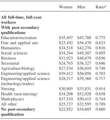
Table 6 reports average 1990 earnings by sex and field
171
P.
Christie,
M.
Shannon
/
Economics
of
Education
Review
20
(2001)
165–180
Table 5
Average wage and salary income by educational attainment of full-time, full-year workersa
1985 1990
Women Men Ratiob Women Men Ratiob
Less than grade 5 $13,203 $21,574 0.612 $17,633 $27,877 0.633
Grade 5–8 $14,370 $24,851 0.578 $17,530 $30,192 0.581
Grade 9–13 $17,095 $27,682 0.618 $21,232 $33,195 0.640
High school graduate: no further education $19,085 $29,474 0.648 $23,822 $36,189 0.658 Trades certificate or diploma, no post-secondary $18,580 $30,670 0.606 $24,197 $37,881 0.639 Some non-university post-secondary, no certificate/diploma, not a high school graduate $18,806 $28,943 0.650 $23,645 $34,663 0.682 Some non-university post-secondary, no certificate/diploma, is a high school graduate $19,598 $30,239 0.648 $24,815 $35,946 0.690 Non-university post-secondary, trades certificate $18,871 $30,208 0.625 $23,000 $37,558 0.612 Non-university post-secondary, with certificate/diploma $21,662 $33,020 0.656 $27,380 $40,778 0.671 Some university, no degree, not a high school graduate $21,414 $32,789 0.653 $29,274 $36,853 0.794 Some University, no degree, high school graduate $22,847 $33,515 0.682 $28,294 $41,341 0.684 University, with trades certificate $21,644 $33,741 0.641 $26,737 $41,029 0.652 University, with non-university certificate/diploma $23,695 $33,750 0.702 $30,262 $41,128 0.736 University graduate: other diploma or certificate below Bachelor’s $25,542 $36,599 0.698 $31,937 $44,650 0.715 University graduate: Bachelor’s degree $28,937 $40,077 0.722 $36,440 $49,262 0.740 University graduate: above Bachelor’s $30,882 $42,101 0.734 $40,975 $52,872 0.775 University graduate: professional degree $34,209 $54,414 0.629 $50,859 $66,499 0.765 University graduate: Master’s degree $35,250 $45,089 0.782 $44,904 $56,862 0.790 University graduate: Doctorate $38,866 $49,823 0.780 $49,497 $63,546 0.779
All $20,914 $31,920 0.655 $26,853 $39,655 0.677
a The number of observations in each group is reported in Table 1.
Table 6
Average wage and salary income by field of study, 1990a Women Men Ratiob Fine and applied arts $23,102 $36,470 0.633
Humanities $34,518 $42,276 0.816
Social sciences $34,244 $49,307 0.695
Business $31,923 $48,679 0.656
Secretarial $24,765 $38,327 0.646
Agriculture/biology $27,534 $36,810 0.748 Engineering/applied science $39,412 $56,056 0.703 Engineering/applied science $28,217 $39,360 0.717 (technology/trades)
Nursing $30,905 $33,831 0.914
Health (non-nursing) $34,208 $52,028 0.658 Math/physics $37,510 $50,415 0.744
All other $25,727 $32,595 0.789
No post-secondary $22,852 $34,605 0.660 qualification
a The number of observations for each field is reported in Table 3.
b Women’s average wage and salary as a share of men’s average wage and salary.
of study for all post-secondary graduates. The top paying field for both sexes is engineering, followed, for men by health (other than nursing), math/physics and social sciences and for women by, math/physics then edu-cation.11Fine arts, agriculture/biology and nursing pay
relatively poorly. The female–male earnings ratio is low-est in secretarial, health (other than nursing) business (roughly 0.65–0.66) and fine/applied arts (0.63). The ratio is largest in nursing (0.91), the humanities (0.82) and education (0.78). These rankings are quite similar across age groups. The earnings ratio rose in all fields except nursing and the humanities between 1985 and 1990. Ratios were also higher for younger than older groups in all fields of study.
It is possible to obtain a better idea of the importance of education in explaining the wage gap by recognising that the average wage (w) equals a weighted average of the average wages for each educational grouping i(wi)
where the weights,Pi, are the share of the sample with
level of educational attainmenti. Letting superscriptsm
andfdenote male and female, the earnings gap can then be expressed as follows:
11 Focusing solely on those with university degrees, health becomes the top paying field and business becomes one of the better paying fields.
The second line decomposes the gender gap in average wages into a component attributable to differences in the distribution of men and women across levels of edu-cation and due to differences in average wages for men and women with equal educational attainment.12 This
exercise indicates that only a small part of the gap is attributable to differences in educational attainment — eliminating gender differences in 1990 (by making women’s shares the same as men’s) would raise the earn-ings ratio from 0.677 to 0.680 and close the absolute gap by only $85. Apparently the gap is explained by differences in wages within educational groupings — which will in part reflect gender differences in other earnings-related characteristics.
The apparent unimportance of educational attainment differences within a given year need not imply that trends in the gender earnings gap are unaffected by rela-tive changes in attainment. To assess the effect of attain-ment on trends in the earnings gap a simple set of projec-tions were performed. In the first set, it was assumed that educational attainment levels of 25–34 year-olds in 1990 would eventually spread to older age groupings other things being equal, i.e., taking average wages by attain-ment level and gender as given. This compositional change would increase average earnings for men slightly to $39 764, while those for women would reach $27 660.13 This creates a $700 fall in the size of the
absolute earnings gap and a rise in the earnings ratio from 0.677 to 0.696. A second, similar exercise can be used to project wages backward in time to a point where educational patterns of workers aged 55–64 would apply to all workers age 25 and over. This exercise gives pre-dicted average earnings of $24 512 for women and $37 738 for men and an earnings ratio of 0.650. These simple projections suggest that the ultimate effect of ris-ing educational attainment on the gender gap is more considerable than the role of differences in a particular year suggest.
A decomposition like that in Eq. (1) can also be used to identify the importance of post-secondary graduates’ field of study in explaining the size of the gender wage
12 The decomposition could also be performed by weighting thePm2Pfterms by the average wage for women at each level
of educational attainment. When this is done on our sample the effect of eliminating differences in educational attainment is somewhat larger.
173
P. Christie, M. Shannon / Economics of Education Review 20 (2001) 165–180
gap. Eliminating gender differences in the field of study of post-secondary graduates would close the 1990 gap by $455 and raise the earnings ratio from 0.677 to 0.689. This is a bigger effect than that produced by eliminating differences in educational attainment.14Projecting future
earnings on the assumption that the distribution of fields for 25–34 year-old post-secondary graduates will spread to the older groups, suggests that the gap will fall slightly to $12 428 and the earnings ratio would rise to 0.688 so that future changes in field will have less of an effect than changes in level of attainment.15Projecting
back-wards by applying the pattern of fields for 55–64 year olds to all those 25 and over, gives a gap of $12 954 and an earnings ratio of 0.663 once again less than the effect of the backward projection for attainment levels. Inter-estingly the projections suggest that, despite having a larger impact than attainment differences on the 1990 gender earnings gap, changes in field of study have not been (and will not be) as important as changes in attain-ment in producing changes in the earnings gap.
The projections suggest that past and future changes in educational attainment and field of study have indi-vidually increased the earnings ratio by 0.046 (from 0.650 to 0.696) and 0.025 respectively. To put the size of these changes into perspective, consider that the earn-ings ratio rose by 0.047 over the 1970s and by 0.040 over the 1980s.16 The implied effects of gender differences
in education and changes in educational outcomes are not trivial.
The data on earnings and the projections presented in this section of the paper are very simple. They do not allow, for example, for the influence of characteristics other than education on earnings and may incorrectly measure the earnings effects of education. This is addressed in the following sections of the paper by esti-mation of earnings regressions.
4. Econometric analysis
To isolate the effect of education on the gap in wage and salary income, we estimated log-annual earnings equations and adopted the decomposition techniques associated with Oaxaca (1973) and Cotton (1988). The logarithm of annual wage and salary income was
speci-14 The importance of differences in field of study relative to attainment is a bit surprising, given that the post-secondary graduates represent less than half the sample, however segre-gation index measures do suggest that gender differences in field of study are greater than those in educational attainment. 15 This assumes that the share of post-secondary graduates age 25 and over will rise to that of 25–34 year olds.
16 These figures are taken from Statistics Canada (1996) and are based upon Survey of Consumer Finances data.
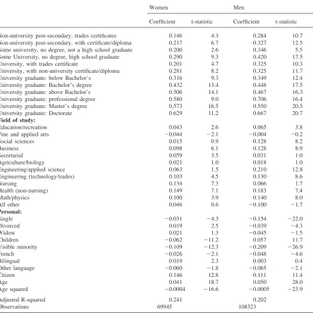
fied to be a linear function of educational attainment, field of study, age and age-squared, personal character-istics (marital and family status, language, visible min-ority, and citizenship), region, urban area, hours of work and industry and occupational dummies. The specifi-cation is similar to earlier Canadian studies using Census data with the exception of the detail of the educational variables. A version of the equation without industry and occupation dummies was also estimated to reflect the concern that the effect of education on wages may, in part, be realised through industry and occupation out-comes. These earnings equations were estimated separ-ately for men and women on the sample of 25–64 year old full-time/full-year workers for both census years. Table 7 reports the results of this exercise for 1990 earn-ings when industry and occupation dummies are included as regressors.
The regression results are quite standard. Wage income rises with age but the effect of an extra year diminishes with age. Wages are lowest in Atlantic Can-ada, Quebec and the Prairies, non-metropolitan areas for those with 30–34 hours per week, visible minorities and non-citizens. Managerial/ professional and teaching occupations have the highest premiums while the lowest paying occupations are farming, clerical (men), service (women) and transportation (women). The pattern for industry coefficients is similar between sexes. Primary industries other than agriculture, communications and utilities and public administration are the best paid. The worst paid are agriculture, services and retail trade.
The default group for educational attainment in the earnings equations is less than grade 5 — the lowest level. For men, coefficients are positive and statistically significant on all education variables in both years. The highest return was associated with professional degrees (medicine, dentistry, etc.), followed by Doctorates, Mas-ter’s and Bachelor’s degrees. Somewhat surprisingly high-school graduates did as well or better than many of those categories with post-secondary education but no university degree. For women, all but one educational attainment coefficient was positive and significant with the largest values for Doctorates, Master’s degrees, then professional degrees. Women with high school degrees typically did as well as those with non-university post-secondary education.
Table 7
Earnings equations estimates for 1990: full-time, full-year, age 25–64 with Industry and Occupation Dummiesa
Women Men
Coefficient t-statistic Coefficient t-statistic
Constant 8.653 158.5 8.572 186.9
Urban 0.127 22.7 0.095 20.9
Region:
Atlantic 20.123 211.9 20.121 214.4
Quebec 20.087 28.8 20.098 211.8
Prairie 20.145 214.9 20.178 221.8
Alberta 20.081 29.4 20.064 29.0
B.C. 20.017 22.1 0.006 0.9
Occupation:
Managerial/administrative 0.233 31.1 0.298 33.4
Natural science 0.208 12.3 0.195 17.8
Social science 0.085 5.7 0.175 9.6
Teaching 0.198 12.7 0.251 14.6
Medicine/health 0.170 13.1 0.211 9.6
Arts/recreation 0.046 2.0 0.092 4.8
Sales 0.041 3.9 0.108 10.4
Service 20.156 214.7 0.061 5.5
Farming 20.364 210.3 20.150 26.7
Primary occupation 0.145 1.1 0.147 6.5
Processing 20.062 22.7 0.114 8.8
Machining 20.128 28.3 0.058 5.9
Construction 0.105 2.2 0.093 8.1
Transport 20.158 24.3 0.010 0.9
Other 20.102 25.9 0.035 3.2
Industry:
Agriculture 20.640 222.5 20.652 233.5
Other primary 0.051 1.8 0.170 11.7
Manufacturing 20.127 211.0 20.037 24.4
Construction 20.188 28.7 20.136 212.1
Transport 20.084 24.3 20.009 20.8
Communications 0.045 3.1 0.061 5.7
Wholesale trade 20.166 211.2 20.092 28.9
Retail trade 20.376 233.1 20.259 226.9
Finance, insurance, real estate 20.141 213.2 20.082 27.4
Business services 20.152 212.1 20.142 213.3
Education services 20.080 25.9 20.137 210.4
Health services 20.197 218.2 20.265 218.8
Accommodation and food 20.441 229.6 20.469 233.2
Other services 20.348 226.1 20.309 225.5
Hours:
Hours 35–39 0.222 24.3 0.149 11.1
Hours 40–44 0.214 23.7 0.154 12.0
Hours 45+ 0.236 22.7 0.205 15.8
Education:
Grade 5–8 20.011 20.4 0.134 5.8
Grade 9–13 0.124 4.3 0.263 11.9
High-school graduate: no further education 0.205 7.0 0.350 15.6
Trades certificate or diploma, no post-sec. 0.172 5.0 0.266 9.9
Some non-university post-secondary, no certificate/diploma, 0.188 5.7 0.302 11.6 not a high school graduate
Some non-university post-secondary, no certificate/diploma, 0.232 7.6 0.364 15.1 is a high school graduate
175
P. Christie, M. Shannon / Economics of Education Review 20 (2001) 165–180
Table 7 (continued)
Women Men
Coefficient t-statistic Coefficient t-statistic Non-university post-secondary, trades certificates 0.146 4.3 0.284 10.7 Non-university post-secondary, with certificate/diploma 0.217 6.7 0.327 12.5 Some university, no degree, not a high school graduate 0.200 2.6 0.346 5.5
Some University, no degree, high school graduate 0.290 9.3 0.420 17.5
University, with trades certificate 0.201 4.7 0.325 10.3
University, with non-university certificate/diploma 0.281 8.2 0.325 11.7
University graduate: below Bachelor’s 0.316 9.3 0.349 12.4
University graduate: Bachelor’s degree 0.432 13.4 0.448 17.5
University graduate: above Bachelor’s 0.506 14.1 0.467 16.3
University graduate: professional degree 0.580 9.0 0.706 16.4
University graduate: Master’s degree 0.573 16.5 0.550 20.5
University graduate: Doctorate 0.629 11.2 0.667 20.7
Field of study:
Education/recreation 0.043 2.6 0.065 3.8
Fine and applied arts 20.044 22.1 20.004 20.2
Social sciences 0.015 0.9 0.128 8.2
Business 0.098 6.1 0.128 8.9
Secretarial 0.059 3.5 0.031 1.0
Agriculture/biology 0.021 1.0 0.018 1.0
Engineering/applied science 0.063 1.5 0.210 12.8
Engineering (technology/trades) 0.103 4.5 0.130 8.6
Nursing 0.134 7.3 0.066 1.7
Health (non-nursing) 0.149 7.1 0.183 7.4
Math/physics 0.100 3.9 0.140 8.0
All other 0.046 0.6 20.100 21.7
Personal:
Single 20.031 24.3 20.154 222.0
Divorced 0.019 2.5 20.039 24.3
Widow 0.021 1.3 20.045 21.5
Children 20.062 211.2 0.057 11.7
Visible minority 20.109 212.3 20.209 226.9
French 20.026 22.1 20.048 24.6
Bilingual 0.019 2.3 0.003 0.4
Other language 20.060 21.8 20.065 22.1
Citizen 0.146 12.8 0.111 11.4
Age 0.041 18.7 0.050 28.0
Age squared 20.0004 216.6 20.0005 223.9
Adjusted R-squared 0.241 0.202
Observations 69945 108323
a Defaults: Occupation: clerical; Industry: public administration; Education: less than grade 5; Field of study: humanities; Region; Ontario.
there are more educational levels at which the coef-ficients for women are larger than for men.17
For field of study of post-secondary graduates humani-ties was the default. Women with health fields did best, ceteris paribus, followed by those in technology/trades
17 Further comparison of the 1985 and 1990 results suggests a fall in returns to education — which was especially large for women. A closer look reveals that the coefficients on the educational attainment dummies have not changed much rela-tive to high school. This suggests that the apparent lower returns
and mathematics/physical sciences. Fine and applied arts and the humanities were the worst paid. The worst paid fields were the same for men as for women. For men, engineering and health paid most.
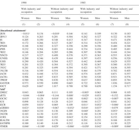
Dropping occupation and industry dummies from the specification (columns 3 and 4, 7 and 8 of Table 8) increases the size of the coefficients on education for
Table 8
Education Coefficient Estimates, 1990 and 1985
1990 1985
With industry and Without industry and With industry and Without industry and
occupation occupation occupation occupation
Women Men Women Men Women Men Women Men
(1) (2) (3) (4) (5) (6) (7) (8)
Educational attainmenta
GR58 20.011c 0.134
20.010c 0.146 0.141 0.189 0.130 0.183
GR913 0.124 0.263 0.201 0.304 0.262 0.327 0.322 0.350
HS 0.205 0.350 0.348 0.413 0.347 0.414 0.471 0.458
TRD1 0.172 0.266 0.327 0.267 0.314 0.270 0.454 0.221
SPNHS 0.188 0.302 0.327 0.358 0.290 0.356 0.400 0.388
SPHS 0.232 0.364 0.401 0.444 0.334 0.418 0.485 0.481
TRD2 0.146 0.284 0.285 0.286 0.307 0.306 0.444 0.244
PSNCD 0.217 0.327 0.409 0.378 0.371 0.363 0.553 0.363
SUNHS 0.200 0.346 0.439 0.444 0.397 0.453 0.556 0.520
SUHS 0.290 0.420 0.504 0.527 0.442 0.469 0.629 0.555
TRD3 0.201 0.325 0.384 0.372 0.395 0.367 0.580 0.353
UNUC 0.281 0.325 0.499 0.394 0.421 0.371 0.636 0.395
UNLTB 0.316 0.349 0.554 0.414 0.464 0.379 0.702 0.405
BACH 0.432 0.448 0.723 0.558 0.574 0.497 0.871 0.557
BACH+ 0.506 0.467 0.833 0.585 0.581 0.520 0.921 0.576
UPROF 0.580 0.706 0.830 0.729 0.637 0.803 0.893 0.784
MASTER 0.573 0.550 0.890 0.665 0.722 0.581 1.036 0.635
DOCT 0.629 0.667 1.017 0.788 0.788 0.658 1.154 0.717
Fieldb
EDREC 0.043 0.065 0.111 0.105 20.003c 0.063 0.068 0.105
ARTS 20.044 20.004c
20.144 0.008c
20.029c 0.053
20.152 0.094
SOCSC 0.015c 0.128 0.018c 0.180 0.002c 0.128
20.007c 0.186
BUS 0.098 0.128 0.128 0.215 0.046 0.127 0.041 0.242
SECR 0.059 0.031c 0.069 0.109 0.011c 0.052c
20.006c 0.149 AGRBIO 0.021c 0.018c 20.067 20.032c 0.018c 0.037c 20.079 0.049
ENGIN 0.063c 0.210 0.130 0.309 0.040c 0.201 0.053c 0.314
ENGTR 0.103 0.130 0.155 0.201 0.100 0.139 0.119 0.229
NURS 0.134 0.066c 0.182 0.043c 0.154 0.123 0.152 0.060c
HEALTH 0.149 0.183 0.170 0.192 0.202 0.252 0.168 0.255
MATHPH 0.100 0.140 0.148 0.212 0.116 0.134 0.130 0.225
OTHER 0.046c
20.100c 0.029c
20.066c
20.030c 0.042c
20.089c 0.068c a The default category is less than grade 5. Acronyms are defined in Table 1.
b The default category is humanities. Acronyms are defined in Table 3. c The coefficient is not statistically significant at 1%.
both sexes but much more for women in both years. In fact, education coefficients are larger for women than men at most levels when the industry and occupation dummies are absent. This change suggests that expansion of the range of occupation and industry of work may be a particularly important source of extra returns to edu-cation for women.18Removing industry and occupational
18 Apparently the payoffs to men of the same education level are more equal across industry/occupations than for women.
dummies also tends to increase the absolute value of the coefficients on the field of study variables.
177
P. Christie, M. Shannon / Economics of Education Review 20 (2001) 165–180
dummies. Similarly coefficients on Grades 5–8 and Grades 9–13 have quite different size coefficients across specifications. In many Canadian surveys these categor-ies would be aggregated into a single “some secondary education” grouping. The restrictions required to sim-plify our 19 category educational variable to a seven cat-egory variable, similar to that found in the Labour Mar-ket Activity Survey (LMAS), were tested and rejected for both sexes and each year.19Tests of the joint
signifi-cance of the field of study variables also suggest that they contribute to explaining variation in earnings.20
Apparently, the greater detail adds significantly to the ability of the regressions to explain variation in earnings.
5. Decomposition of the wage gap
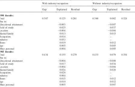
The average log-earnings gap was 0.434 in 1985 for full-time, full-year workers. This had fallen to 0.387 by 1990. The first row of Table 9 reports the decomposition of the 1990 gender wage gap into explained and residual components along the lines of Oaxaca (1973):
wm
whereXis a vector of average values of wage-determin-ing characteristics, b is the vector of coefficients obtained by regressing the log-wage on the variables in
Xand, as before,m andf superscripts denote male and female respectively. The first term of the equation meas-ures that part of the gap explained by gender differences in average characteristics. The second term is the residual component which accounts for differences in unobservable characteristics and wage discrimination. The first term in Eq. (2) is often interpreted as the size of the wage gap if there were no discrimination. Under this interpretation Eq. (2) uses male wage coefficient estimates as the proxy for wage structure in the absence of discrimination. This choice is somewhat arbitrary and the results are potentially sensitive to this choice. Cotton (1988) suggests that a weighted average of male and female wage coefficient estimates (bc) may be a more
reasonable no-discrimination proxy.21 Cotton’s
decomposition gives:
19 For 1990, with industry and occupation dummies the test statistics were F(20, 69877)=15.8 for women and F(20, 108255)=26.1 for men. The specifications used to test these attainment restrictions excluded field dummies.
20 TheF-tests for the joint significance of the field variable coefficients gave F(12, 69865)=13.8 for women and F(12, 108243)=27.7 for men in 1990 with industry and occupation dummies present.
21 The weights are simply the male and female shares of the combined wage equation samples.
where the first term is the explained component, now evaluated usingbcrather thanbm, the second term
meas-ures the male residual or treatment advantage and the last term the female residual or treatment disadvantage. Taken together the last two terms are the counterpart of Oaxaca’s residual effect. Results of the Cotton decompo-sition are reported in Table 10.
We look first at the Oaxaca decomposition results. For 1985 with industry/occupation variables included, 0.155 of the log-earnings gap (36%) can be explained by differ-ences between men and women in the average level of earnings-determining characteristics and 0.279 is due to differences in payoffs to these characteristics for men and women (see the second part of Table 9). In 1990, 0.125 (32%) was explicable in terms of different average characteristics and 0.261 due to different payoffs. The differences in component size between the two years suggests that relative improvements in earnings-determining characteristics accounted for about one half of the fall in the measured gap. Further decomposition of the explained component reveals that gender differ-ences in industry of employment are the largest contribu-tor to the explained portion of the gap in both years. This is followed by occupation in 1985 and field of study in 1990. Differences in educational attainment by gender had little effect on the explained component in either year, while differences in field of study accounted for 0.017 of the explained component in 1985 and 0.025 in 1990.22As Oaxaca and Ransom (1999) point out, a
simi-lar decomposition of the residual component by charac-teristic is sensitive to the choice of dummy variable ref-erence groups and therefore unreliable — consequently it is not reported.
When industry/occupational dummies are left out of the specification the picture changes substantially. The explained component falls by nearly half. Differences in the field of education become a more important determi-nant of the size of the diminished explained component in both years. In both sets of results, the greater relative importance of differences in field of study compared to differences in attainment is consistent with the results in Section 3.23
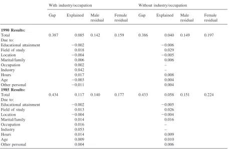
When the Cotton decomposition is used in place of
22 On a sample of university graduates Wannell (1990) also found that differences in field were more important in explaining the wage gap than differences in levels.
Table 9
Oaxaca decomposition of the gender earnings gap, full-time year workers in 1990 and 1985a
With industry/occupation Without industry/occupation
Gap Explained Residual Gap Explained Residual
1990 Results:
Total 0.387 0.125 0.261 0.386 0.062 0.324
Due to:
Educational attainment 20.003 20.007
Field of study 0.025 0.037
Location 20.004 20.004
Marital/family 0.013 0.015
Occupation 0.014 –
Industry 0.053 –
Hours 0.019 0.012
Age 0.005 0.005
Other personal 0.004 0.005
1985 Results:
Total 0.434 0.155 0.279 0.433 0.079 0.354
Due to:
Educational attainment 20.004 20.008
Field of study 0.017 0.034
Location 20.004 20.004
Marital/family 0.024 0.028
Occupation 0.028 –
Industry 0.064 –
Hours 0.015 0.012
Age 0.010 0.012
Other personal 0.005 0.007
a Oaxaca decomposition: see Eq. (2).
the Oaxaca decomposition, the explained component is smaller in all years and specifications. However, in all other respects the results are quite similar. The explained component is smaller when industry and occupational dummies are left out, educational attainment remains an unimportant contributor to the explained component while field of study contributes positively and is especially important in the absence of industry and occu-pational dummies. The major new insight provided by the Cotton decomposition is its breakdown of the residual into a male advantage and female disadvantage component. The latter term accounts for most of the residual term in all years and specifications. Over time the fall in the combined residual term reflects a decline in the female disadvantage term.
Projections of future and past log-wage levels, along the lines of those presented in Section 3, were made based upon the earnings regression estimates. Under the assumption that in the future educational attainment and field of study patterns of older workers converge to that of 25–34 year olds, the 1990 gap changes from 0.387 to 0.361 when industry/occupation dummies were present or 0.350 when the latter were absent. If, projecting back-wards in time, the 55–64 year old patterns were to
pre-vail for workers age 25 and older, the gap would be 0.386 (with industry/occupation) or would climb to 0.406 (no industry/occupation). As in Section 3, these changes are driven by the changes in educational attain-ment.
6. Comparison with previous studies
How important is the extra educational detail provided in the Census to the decomposition of the gender gap? The results clearly suggest that having data on field of study aids in explaining the gap. In both years, differ-ences by gender in field of post-secondary qualification account for a significant part of the earnings gap. The highest estimate (the 1990 results with no industry and occupation dummies) is nearly 10% of the total gap and over half of the explained component. Field of study was typically either unavailable or not controlled for in earl-ier Canadian studies.
179
P. Christie, M. Shannon / Economics of Education Review 20 (2001) 165–180
Table 10
Cotton decomposition of the gender earnings gap, full-time year workers in 1990 and 1985a
With industry/occupation Without industry/occupation
Gap Explained Male Female Gap Explained Male Female
residual residual residual residual
1990 Results:
Total 0.387 0.085 0.142 0.159 0.386 0.040 0.149 0.197
Due to:
Educational attainment 20.002 20.006
Field of study 0.018 0.029
Location 20.004 20.005
Marital/family 0.006 0.006
Occupation 0.002 –
Industry 0.042 –
Hours 0.017 0.008
Age 20.003 0.004
Other personal 20.011 0.004
1985 Results:
Total 0.434 0.117 0.140 0.177 0.433 0.058 0.151 0.224
Due to:
Educational attainment 20.002 20.005
Field of study 0.013 0.026
Location 20.004 20.004
Marital/family 0.014 0.016
Occupation 0.016 –
Industry 0.053 –
Hours 0.014 0.009
Age 0.009 0.010
Other personal 0.004 0.006
a Cotton decomposition: see Eq. (3).
Stelcner (1987) and Miller (1987), using Census data for 1980 all find that differences in educational attainment explain virtually none of the gap — consistent with our results. Estimates by Doiron and Riddell (1994) for 1984 (Survey of Union Membership) and Kidd and Shannon (1995) for 1981 (Survey of Work History) and 1989 (LMAS) suggest the same result for gender differences in average log-hourly wages.24The apparent
unimport-ance of the additional detail on educational attainment is confirmed by re-estimating our earnings equations using a simpler 7-category attainment variable (differences in attainment account for 20.003 to 20.008 of the gap depending on year and specification).
Our results largely parallel those for the US. Education variables used in the US literature are often quite simple. Years of schooling, sometimes augmented by a dummy for college degree are common. Consistent with Canad-ian results, differences in the quantity of schooling appear to play little role in explaining gender differences in wages, see for example Blau, Ferber and Winkler
24 The result is derived from the 1984 regression results and means table reported in Doiron and Riddell (1994).
(1998, p. 190) who report that educational attainment differences accounted for only 0.3 of the 27.6 percentage point gap in 1988.25The US literature also provides
evi-dence of the importance of field of study. Brown and Corcoran (1997) find that field of study accounts for 0.08–0.09 of the 0.21 gender wage gap for a sample of college educated workers. They also note that, as for our results, the importance of field of study declines with the inclusion of industry and occupational dummies. An earlier study of recent college graduates by Daymont and Andrisani (1984) gave similar results with field of study explaining 0.045–0.058 of a 0.129 gap. These effects are somewhat larger than those obtained on our subset of university educated workers (see23).
7. Conclusions
Using the detailed data on education from the Canad-ian Census the paper documents substantial gender dif-ferences in educational attainment and field of study of post-secondary graduates. Our results suggest that allowing for greater educational detail does help explain variation in wages. Differences in educational attainment do not help explain the earnings gap in 1985 or 1990 — a result also found in earlier studies using less detailed educational attainment data. Differences in field of study are more helpful, using the Oaxaca decomposition they explain 0.025 to 0.037 of the 1990 log-earnings gap of 0.387.
Projections suggest that changes over time in field of study and, more importantly, educational attainment have closed and will continue to close the gender earn-ings gap. The largest estimates suggest that changing educational outcomes may have lowered the gap from 0.406 to 0.387 and could drive it as low as 0.350 in the future.
Appendix A. Education in Canada
Education in Canada is the responsibility of the ten Provincial governments. In practice, the general structure of education is quite similar across provinces. However some differences exist, the most important concerning the number of grade levels in the elementary-secondary system, the existence of public pre-school programs, the role of Catholic and other religious schools and the requirements for admission to university. Students typi-cally start elementary education at age 5–6, sometimes after 1–2 years of pre-school kindergarten. The elemen-tary–secondary level of education typically consists of 12 grades each of which takes one year to complete (the largest province, Ontario, had 13 grades until recently while Quebec had only 11). A high-school graduate is someone who has successfully completed secondary school.
Non-university post-secondary institutions include community colleges, CEGEPs (in Quebec), agricultural, art, teacher and nursing schools. These institutions pro-vide career oriented programs at the post-secondary level which can vary from 1–4 years in length. Sufficiently qualified secondary school graduates may, upon accept-ance by the relevant institution, enter university (in Que-bec two years study at a CEGEP is also required). Bach-elor’s level degrees typically take 4 years to complete. Professional studies at the university level are entered after completion, or in some cases, after partial com-pletion of a Bachelor’s degree.
Trades education, which provides occupation specific training, may be offered at secondary or post-secondary levels and in the case of apprenticeship may involve a substantial on-the-job component.
References
Baker, M., Benjamin, D., Desaulniers, A., & Grant, M. (1995). The distribution of the male/female earnings differential, 1970-1990.Canadian Journal of Economics,28, 479–501. Blau, F., Ferber, M., & Winkler, A. (1998).The economics of women, men and work.(3rd ed). Upper Saddle River: Pren-tice-Hall.
Brown, C., & Corcoran, M. (1997). Sex-based differences in school content and the male-female wage gap.Journal of Labor Economics,15, 431–461.
Cotton, J. (1988). On the decomposition of wage differentials. Review of Economics and Statistics,70, 236–243. Daymont, T., & Andrisani, P. (1984). Job preferences, college
major, and the gender gap in earnings.Journal of Human Resources,19, 403–428.
Doiron, D., & Riddell, C. (1994). The impact of unionization on male-female earnings differences in Canada.Journal of Human Resources,XXIX(2), 504–534.
Gunderson, M. (1979). Decomposition of the male/female earn-ings differential: Canada 1970. Canadian Journal of Eco-nomics,12, 479–485.
Kidd, M., & Shannon, M. (1995). The gender wage gap in the 1980s. Presented at Canadian Economics Association Meet-ings, Montreal.
Macpherson, D., & Hirsch, B. (1995). Wages and gender com-position: why do women’s jobs pay less?Journal of Labor Economics,13, 426–471.
Miller, P. (1987). Gender Differences in Observed and Offered Wages in Canada, 1980.Canadian Journal of Economics, 20, 225–244.
Neumark, D. (1988). Employers’ discriminatory behavior and the estimation of wage discrimination. Journal of Human Resources,23, 279–295.
Oaxaca, R. (1973). Male-female wage differentials in urban lab-our markets.International Economic Review,14, 693–709. Oaxaca, R., & Ransom, M. (1999). Identification in detailed wage decompositions.Review of Economics and Statistics, 81, 154–157.
Shapiro, D., & Stelcner, M. (1987). The persistence of the male-female earnings gap in Canada, 1970–1980: the impact of equal pay laws and language policies.Canadian Public Pol-icy,13, 463–476.
Sorenson, E. (1989). The crowding hypothesis and comparable worth.Journal of Human Resources,25, 55–89.
Statistics Canada (1996).Earnings of men and women in 1996. Catalogue 13-217-XPB.Ottawa: Industry Canada. Wannell, T. (1990). Male-female earnings gap among recent