www.elsevier.comrlocateratmos
Optical and microphysical parameters of dense
stratocumulus clouds during mission 206 of
EUCREX ’94 as retrieved from measurements
made with the airborne lidar LEANDRE 1
J. Pelon
a,), C. Flamant
a, V. Trouillet
a, P.H. Flamant
ba
SerÕice d’Aeronomie du CNRS, 4 Place Jussieu, B 102, F-75252 Paris, France´
b
Laboratoire de Meteorologie Dynamique, France´ ´
Received 4 December 1999; accepted 1 March 2000
Abstract
Cloud parameters derived from measurements performed with the airborne backscatter lidar LEANDRE 1 during mission 206 of the EUCREX ’94 campaign are reported. A new method has been developed to retrieve the extinction coefficient at the top of the dense stratocumulus deck under scrutiny during this mission. The largest extinction values are found to be related to the highest cloud top altitude revealing the small-scale structure of vertical motions within the
Ž .
stratocumulus field. Cloud optical depth COD is estimated from extinction retrievals, as well as cloud top and cloud base altitude using nadir and zenith lidar observations, respectively. Lidar-derived CODs are compared with CODs deduced from radiometric measurements made onboard the French research aircraft Avion de Recherche Atmospherique et de Teledetection´ ´ ´ ´
ŽARATrF27 . A fair agreement is obtained within 20% for COD’s larger than 10. Our results. Ž . show the potential of lidar measurements to analyze cloud properties at optical depths larger than 5.q2000 Elsevier Science B.V. All rights reserved.
Keywords: Lidar; Stratocumulus; Cloud microphysics; Cloud optical properties
1. Introduction
Stratocumulus clouds are frequently observed in mid- and high latitudes to extend over large oceanic areas. They significantly reduce the solar flux reaching the surface,
)Corresponding author. Tel.:q33-1-44-27-37-79.
Ž .
E-mail address: [email protected] J. Pelon .
0169-8095r00r$ - see front matterq2000 Elsevier Science B.V. All rights reserved.
Ž .
( ) J. Pelon et al.rAtmospheric Research 55 2000 47–64
48
and increase the earth–atmosphere albedo. As they weakly modify the upward longwave
Ž
fluxes, their occurrence results in a strong modification of the radiation budget net
.
cooling . Marine and continental stratocumulus are known to have different
microphysi-Ž .
cal properties Martin et al., 1994 and, in turn, different impact on the shortwave
Ž .
radiation budget at the global scale Kiehl, 1994 . Measuring modifications in their characteristics is thus a critical issue with respect to climate change. This point has been emphasized by the potential impact of aerosol on cloud nucleation, the so-called indirect
Ž .
radiative forcing of aerosol Twomey, 1977; Boucher and Lohman, 1995 . The retrieval of stratocumulus optical and microphysical properties at the global scale is, thus, an important step towards the understanding of their radiative impact. To this respect, the
Ž .
most significant parameters are the cloud structure cloud fraction, top and base heights , the effective radius and the liquid water content which control cloud optical depth
ŽCOD. ŽZhang et al., 1995 . In situ measurements provide accurate measurements of.
such parameters. However, they are only obtained over selected areas during field campaigns. Remote sensing is the only way to derive quantitative information about the occurrence of clouds and their properties at scales large enough to be used as inputs in general circulation models. Retrieval of cloud parameters using such techniques as
Ž .
aimed at in EUCREX ’94 Raschke et al., 1997 is thus, of importance. Passive
measurements have been widely used for such a purpose. However, it has been shown that the retrieval of cloud properties using standard techniques may be biased due to the
Ž .
presence of overlying semi-transparent clouds Doutriaux et al., 1998 and to spatial
Ž .
cloud inhomogeneity Fouquart et al., 1990; Cahalan et al., 1994 .
Active remote sensing by lidar appears to be a promising tool for complementary
Ž .
cloud parameter analysis at the global scale Doutriaux et al., 1998 . However, stratocu-mulus clouds being optically dense, they, most of the time, preclude lidar observations over their whole vertical extent. Thus, the COD cannot be determined using standard
Ž
inversion procedures as used for semi-transparent clouds Carnuth and Reiter, 1986;
.
Flamant et al., 1996 . Up to now, airborne backscatter lidar have been used to analyze microphysical properties of moderately dense stratocumulus cloud at the meso-scale in
Ž .
complement to passive observations Spinhirne et al., 1989 .
The objectives of the EUCREX ’94 campaign were focused on the retrieval of optical and microphysical properties of both high and low cloud by means of remote sensing. The French airborne lidar LEANDRE 1 was one of the components of the experimental setup. Lidar observations were made from one of the French research aircraft, the Avion
Ž .
de Recherche Atmospherique et de Teledetection ARAT
´
´ ´ ´
rF27 . Results from flightsŽ
dedicated to the study of cirrus clouds have been presented elsewhere Sauvage et al.,
.
1999; Chepfer et al., 1999 .
The scope of this paper is to present the procedure developed to improve lidar signal
Ž y3
analysis in dense clouds typically characterized by water contents larger than 0.3 g m
.
and optical depth larger than 10 and present cloud parameters obtained by lidar on the
Ž .
case study of mission 206 18 April 1994 of EUCREX ’94 selected for the analysis of
Ž
stratocumulus properties using remote sensing and in situ techniques Brenguier and
.
Lidar-derived CODs are discussed in Section 4 in connection with those derived from visible fluxes measured simultaneously by passive radiometers onboard the ARAT. Liquid water content derived from the lidar data analysis in convective cells is used to
Ž .
derive an estimate of droplet concentration and effective radius at cloud top Section 5 . The cloud parameters retrieved from the lidar data will be further compared to other estimates from in situ and remote sensing instruments in the conclusion paper of the
Ž .
series Pawlowska et al., 2000b .
2. Airborne measurements
A high pressure system was centered over England bringing cold subsiding air from
Ž
northern Europe over the north-western part of France see Section 4 and Fig. 2 of
.
Brenguier and Fouquart, 2000 . The structure of cloud radiance observed by AVHRR at
Ž .
08:30 UTC in the visible channel is given in Fig. 1 of Fouilloux et al., 2000 .
Ž . Ž .
( ) J. Pelon et al.rAtmospheric Research 55 2000 47–64
50
Stratocumulus, characterized by higher radiance values are seen to extend over the
Ž .
English Channel, eastern England and over western Brittany France . Flights were
Ž .
performed by the ARAT on a leg AM about 100 km long, northwest of Brittany above
Ž .
this cloud deck see Fig. 1 in Brenguier and Fouquart, 2000 . AVHRR radiances revealed that the stratocumulus deck was breaking west of point A and did not extend very far beyond this point. The track was flown eight times between these two points.
Ž .
Once between 9:15 and 9:40 UTC, at a level of 300 m further referred to as AM1 to
Ž .
document cloud properties from below cloud base height and extinction , and seven times at a level of 4500 m between 9:58 and 12:18 UTC to retrieve cloud top height and
Ž
extinction coefficient as would be obtained from a space-borne system Table 1 in
.
Brenguier and Fouquart, 2000 . In this study, we focus on the second AM and MA legs
Ž .
flown by the ARAT further referred to as AM2 and MA2 between 10:34 and 10:54
Ž .
UTC, and 10:57 and 11:17 UTC Table 1 in Brenguier and Fouquart, 2000 .
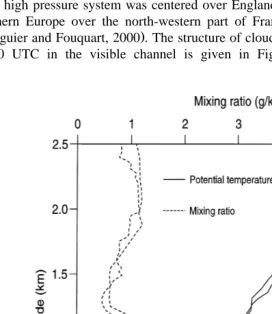
The vertical potential temperature and humidity profiles measured during ARAT ascent and descent near points M and A, at 9:40 and 12:10 UTC, respectively, are reported on Fig. 1. They show a significant evolution in the vertical structure along the leg defined by these two points, and during the mission, as the temperature inversion height decreases from about 1000 to 800 m going from M to A. The values of water vapor mixing ratio in the upper mixed boundary layer are comparable at both points, about 4.1 and 4.3 g kgy1 in A and M, respectively. A 1.2-K increase in temperature is
Ž .
observed between A and M. The lifting condensation level LCL calculated from these values corresponds to an altitude of about 600 m. These observations are in agreement
Ž
with those obtained by the Merlin IV see Pawlowska et al., 2000a, which is further
. Ž
referred to as PBB . The visible image obtained from AVHRR see Fouilloux et al.,
.
2000 showed that the radiance values were much larger near M, emphasizing the increased reflectance and optical depth of the cloud deck closer to the coast.
3. Lidar data analysis
The ARAT was embarking the backscatter lidar LEANDRE 1. This airborne system
Ž .
uses a pulsed Nd–Yag laser source, emitting in the visible spectral domain 532 nm after frequency doubling. A specific channel is also used for the detection of the signal
Ž .
at the fundamental wavelength 1.06mm . This airborne lidar has been used to retrieve atmospheric aerosol, boundary layer characteristics and cloud scattering properties
Ž
during previous campaigns Flamant and Pelon, 1996; Valentin et al., 1994; Flamant et
. Ž .
al., 1998 . In standard analysis procedures, the lidar signal S z, t , obtained as a function of distance z and time t, is first processed to derive the attenuated backscatter
Ž .
coefficient ba z defined as the product of the real atmospheric backscatter coefficient
2Ž .
bz with the two-way transmission T z between the aircraft and the particles
Ž
scattering the lidar beam at a given time or distance z see Spinhirne et al., 1989 for
.
3.1. Cloud boundary analysis
Lidar signal is normalized to atmospheric scattering at an altitude close to the aircraft,
Ž .
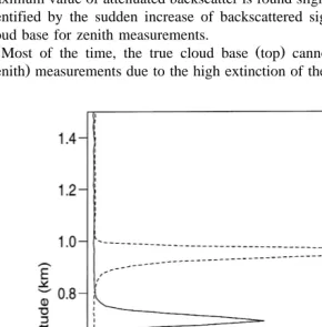
using onboard nephelometer measurements Flamant et al., 1998 . Fig. 2 shows two attenuated backscatter profiles obtained in nadir and zenith viewing mode. Larger ba
values correspond to cloud scattering. Zenith measurements were taken as the aircraft was flying at 300 m above sea level. These vertical profiles have been obtained with a vertical resolution of 15 m and a horizontal resolution of 100 m, corresponding to an
Ž .
acquisition time of 1 s 12 laser shots . During the low-level leg, the overlap between emitted and received beams prevented from getting valid information below 450 m.
Attenuated backscatter profiles obtained in nadir viewing show that the lidar signal is
Ž .
rapidly decreasing as the beam penetrates into the cloud Fig. 2 . Therefore, the
Ž
maximum value of attenuated backscatter is found slightly under the cloud top which is
.
identified by the sudden increase of backscattered signal . The same is applicable to cloud base for zenith measurements.
Ž .
Most of the time, the true cloud base top cannot be observed from such nadir
Žzenith measurements due to the high extinction of the lidar beam caused by scattering.
()
J.
Pelon
et
al.
r
Atmospheric
Research
55
2000
47
–
64
52
Ž . Ž . Ž .
Ž .
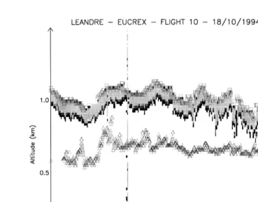
into the cloud the transmission rapidly decreases to zero . This is emphasized in Fig. 3,
Ž . Ž
which shows the retrievals of cloud top square and apparent cloud base lower limit of
. Ž .
the grey area altitudes from nadir measurements, and of cloud base altitude triangle from zenith measurements, as a function of the position of the aircraft along the leg MA. AAthresholdB algorithm based on the detection of the lidar signal gradient change was
Ž .
used to derive cloud base and top heights Trouillet, 1997 from nadir and zenith measurements. The cloud top altitude can be precisely derived from nadir viewing due to the large signal gradient observed near the cloud top and the lack of attenuation above. Due to attenuation, the cloud base altitude derived from zenith measurements is fairly different from the apparent base defined with the same threshold from nadir
Ž .
measurements 650 m instead of 900 m, Fig. 2 . Only close to point A is the apparent cloud base deduced from nadir measurements close to the one obtained from zenith. In this area, COD is decreasing, and clear air areas are even observed in downdrafts, as shown from increased attenuated backscatter coefficients from below the cloud base.
Ž
Surface returns are also detected near point A i.e. the beam is not completely attenuated
.
in the cloud . The surface echo also gives an absolute altitude reference to within 10 m. The cloud base altitude is seen to correspond to 650 m. This is in good agreement
Ž .
with the altitude determined from in situ measurements see PBB , and is very close to the LCL height obtained from the soundings. The cloud top height analyzed on this leg
ŽFig. 3 is seen to decrease from values larger than 1100 m to less than 800 m from M to.
A. It exhibits a larger variability than expected from the temperature soundings given in
Ž
Fig. 1. Small-scale variability is also important with variations of the cloud top height
.
greater than 100 m over a 5-km horizontal distance and reveals intense convective
Ž
motions into the cloud at this scale. The cloud base height zb varies slightly between
.
620 and 680 m , and was taken to be equal to 650 m in the rest of the study. The cloud geometrical depth is further referred to this value.
3.2. Analysis of cloud optical properties
In moderately dense clouds, optical properties can be analyzed from the attenuated
Ž
backscatter coefficient while accounting for multiple scattering Carnuth and Reiter,
.
1986; Spinhirne et al., 1989; Flamant et al., 1996 . In dense clouds, however, the detection bandwidth may significantly contribute to the signal amplitude limitation, and this effect needs to be corrected for in the case of rapidly varying signals. In direct detection, the detected lidar signal is proportional to the optical power backscattered by the atmosphere. It can be written as the double convolution of the laser pulse power
Ž .
P te emitted as a function of time t, with the impulse response of the atmosphere
Ž . 2 Ž .
ba z rz as a function of altitude z, and the detection response D t
ba
S z ,t
Ž
.
sKs 2Ž .
z mP teŽ .
qPbŽ .
t mD tŽ .
qSbŽ .
t ,Ž .
1z
where Pb and Sb are additive optical and electrical noises, respectively. Ks is the overall detection efficiency of the lidar system. The value of this efficiency factor is determined during upper level flights with reference to molecular and particular
extinc-Ž
tion measured onboard the ARAT with a transmission nephelometer Flamant et al.,
.
( ) J. Pelon et al.rAtmospheric Research 55 2000 47–64
54
The duration of the pulse emitted by the LEANDRE 1 laser source being very short when compared to the signal sampling time constant, only the second convolution in Eq.
Ž .1 needs to be considered. This convolution can be calculated using a simple formalism, which requires the knowledge of the detection bandwidth and of the multiple scattering contribution. The latter can be estimated from the attenuated backscatter coefficient
Ž . Ž
ba z , integrated over the cloud depth following previous analysis Platt, 1973;
Spin-.
hirne et al., 1989 , and accounting for the detection filtering. However, a cloud scattering model must be defined for this purpose. We have chosen to represent the cloud edge by a steep increase in the scattering and extinction coefficients. The transition zone at cloud edge thus corresponds to a time propagation of light much smaller than the equivalent time constant of the detection system. The backscatter and
Ž .
extinction coefficients and consequently, their ratio k are kept constant in the first tens of meters below the cloud top. Under such hypotheses and assuming a first order frequency response of the detection system, the in-cloud attenuated backscatter
coeffi-) Ž ) .
where zS is the equivalent height scale of the detection system corresponding to the
Ž .
electronic bandwidth. Using the formalism proposed by Platt 1973 , multiple scattering in cloud can be represented as a reduction in the real cloud extinction coefficient a by a
Ž . Ž .
factor 1rh h-1 . The first term in Eq. 2 corresponds to the two-way atmospheric
transmission.
Ž .
Calculation of the integrated attenuated backscatter coefficient IAB has been made
as a function of the normalized penetration distance into the cloud z
ˆ
)sz)rzS
Žassuming the same time–distance equivalence as without multiple scattering . The.
Ž .
theoretical expression of IAB obtained from Eq. 2 is given by
ka
) ) )
IAB z
Ž
ˆ
.
s 1yXqXexpyzˆ
yexpyXzˆ
,Ž .
32 1
Ž
yX.
Ž .
where Xs2ahz . Let k be the backscatter to extinction coefficients ratio BER . TheS apparent BER, k , is then defined as krh. For large values of z
ˆ
) and X, the IAB tendsa
towards the asymptotic value kar2. Note that this value is the same as the one
Ž .
calculated for an infinite detection bandwidth zSs0 and that the corresponding
Ž .
expression of the IAB is equivalent to the one obtained by Platt 1973 .
However, the value of X is unknown and the assumption that X is large may be
Ž .
questionable. According to Eq. 2 , this parameter also depends on the apparent
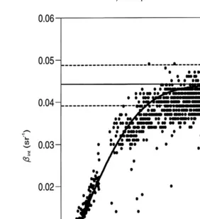
backscatter coefficient. Since there exists an altitude for which the apparent backscatter coefficient is maximum, the IAB is a function of the maximum of apparent backscatter coefficient. This function does not have to be known because the IAB and the maximum of apparent backscatter coefficient can be determined independently. In Fig. 4, the IAB
Ž .
Fig. 4. Integrated attenuated backscatter coefficient as a function of maximum attenuated backscatter
Ž .
coefficient at 532 nm for legs AM2 and MA2.
cloud. As the cloud top temperature is close to 08C, only water droplets are assumed to be found in the cloud. In this case, the BER in the cloud is constant and equal to 0.057
y1 Ž .
sr , independent of the cloud droplet distribution Pinnick et al., 1983 . It can be
shown that the asymptotic value of the IAB is the same for large X and large attenuated
Ž .
backscatter values i.e. kar2 . This allows us to derive the multiple scattering factors, as we now discuss. From Fig. 4, we observe than the IAB tends towards a value of 0.044 sry1. Therefore, the apparent BER is estimated to be k r2s0.044"0.006 sry1. The
a
uncertainty is estimated from the fluctuations around the mean value given by the dotted lines in Fig. 4. The corresponding value of the multiple scattering factor ishs0.62"
Ž .
0.10. It is slightly higher than the one determined by Spinhirne et al., 1989 , most likely
Ž
because clouds were observed with a different solid angle our lidar observations were
.
made closer to the cloud .
Ž .
The true extinction coefficient a at cloud top is then retrieved from Eq. 2 , using the
Ž .
relationship bska and the maximum backscatter coefficient value measured Fig. 4 .
( ) J. Pelon et al.rAtmospheric Research 55 2000 47–64
56
inverse relationship leads to large errors for high extinction coefficient values. An 8% statistical error due to noise in the attenuated backscatter coefficient for example results in a 20% error on a retrieved extinction coefficient of the order of 0.015 my1. The bias is more difficult to estimate. In Fig. 4, it can be seen that for values of ba close to 0.8
y1 y1 Ž .
km sr , there appears to be a slight difference about 10% in the IAB given by the
Ž .
theoretical expression given by Eq. 3 and the experimental points. This may be due to the inadequacy of our simple model to represent cloud extinction, and may lead to an underestimation of medium range extinction.
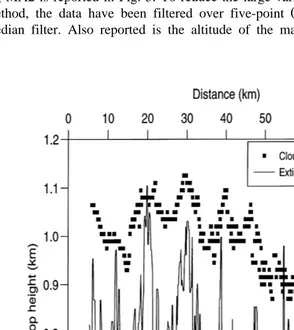
The extinction coefficient at cloud top at, retrieved as a function of distance along leg MA2 is reported in Fig. 5. To reduce the large variability induced by the inversion
Ž .
method, the data have been filtered over five-point total number intervals using a median filter. Also reported is the altitude of the maximum value of the attenuated
Ž .
Fig. 5. Lidar-derived cloud top extinction coefficient at 532 nm solid line and maximum in-cloud apparent
Ž .
backscatter coefficient height dotted line along leg MA2. The retrieval is performed on a 1-s accumulation
Ž .
Ž .
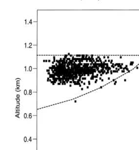
Fig. 6. Vertical distribution of the cloud top extinction coefficient at 532 nm for legs AM2 and MA2. The
Ž .
dotted line represents Eq. 11 . The solid line marks the altitude of the highest cloud observed.
backscatter coefficient. Extinction and altitude simultaneous increases and decreases are indicative of convective cells, already identified in Fig. 3. The correlation coefficient between these two parameters is 0.92. Small-scale fluctuations appear to be more important on the extinction coefficient than on the cloud top altitude. This results in the vertical distribution of the cloud top extinction shown in Fig. 6. Data from legs AM2 and MA2 have been included to emphasize vertical fluctuations of the cloud optical properties caused by the entrainment process at top of the cloud deck. In Fig. 6, 99.9% of the values of the cloud-top height are observed between 1120 and 850 m. The largest value of cloud-top extinction is about 0.17 my1. Precision in the filtered values of the extinction coefficient is expected to be of the order of 10%. This figure is further discussed in Sections 5 and 6.
4. COD
The COD has then been estimated from the retrieved extinction coefficient at cloud
Ž .
( ) J. Pelon et al.rAtmospheric Research 55 2000 47–64
58
for each measurement point, the extinction coefficient was linearly increasing from cloud base up to the value derived at cloud top. This hypothesis is used as an approximation of the ratio of the vertical distribution of the liquid water content and
Ž .
effective radius defining the extinction coefficient as discussed in Section 5 in both
Ž .
upward and downward motions see in situ measurements in PBB . The estimated optical deptht is thus given by
1
)
ts atz ,t
Ž .
42
where a and z) are the extinction coefficient at the top of the cloud and the cloud
t t
geometrical thickness, respectively.
Ž
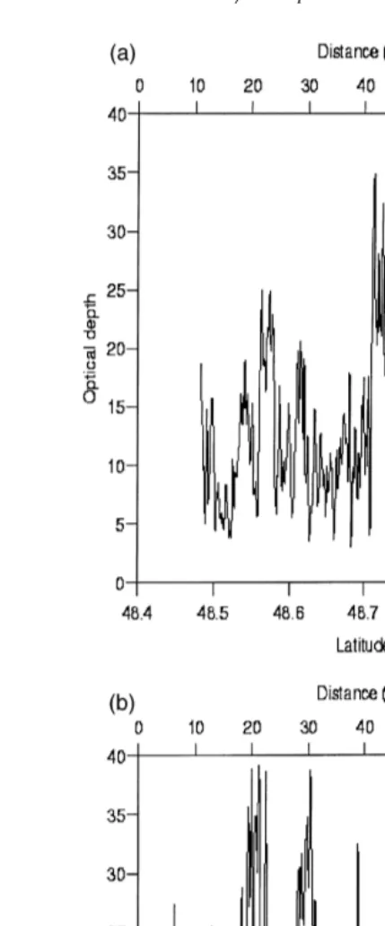
Results from legs AM2 and MA2 are reported in Fig. 7a and b, respectively values
. Ž .
are filtered over 5 points . The convective structures near 48.68N previously identified in Fig. 5 are also clearly evidenced here. CODs as large as 40 are observed in the most
Ž .
energetic updrafts, and a large variability within a factor 3 is observed between updraft and downdraft.
Simultaneously to lidar measurements, the upward and downward shortwave fluxes were measured onboard the ARAT using the broadband visible Eppley pyranometers. A calibration flight performed with the Merlin IV of Meteo–France and the Falcon 20 of
´ ´
DLR was designed to assess the consistency of the visible flux measurements made by the three aircraft. On average, they agreed to within 0.2% as the three aircraft wereŽ .
flying at an altitude of 1.5 km Sauvage et al., 1999 . The plane albedo A of thea
surface–cloud–atmosphere system was deduced from the ratio of the upward and
downward shortwave flux FSW measured by the upward and downward looking
pyranometers as the ARAT flew over the stratocumulus layer
FSW≠
AAs .
Ž .
5FSWx
As data were taken on a constant level leg near noon, no attitude nor solar zenith
Ž .
elevation corrections were made on the measured solar fluxes Saunders et al., 1992 .
Ž .
Albedo values increase from about 0.2 near A to 0.7 near point M not shown for leg MA2. Using a plane-parallel cloud model and assuming no absorption, two-stream approximations in radiative transfer calculations show that the COD,t, can be deduced
Ž .
from the total plane albedo A as Meador and Weaver, 1980A
AA
ts ,
Ž .
6g
Ž
1yAA.
Ž
whereg is a parameter depending on the radiation model used Meador and Weaver,
. Ž .
1980 . In the case of the Eddington scheme, the value ofg is 3r4 1yg , where g is
the asymmetry factor of the cloud droplet distribution. As gs0.85 for water spheres,
we obtain gs8.8. Fig. 8 shows a comparison between the COD derived from the
Ž . Ž
Fig. 7. Estimated cloud optical depth at 532 nm vs. latitude as derived from lidar data filtered extinction
. Ž . Ž .
( ) J. Pelon et al.rAtmospheric Research 55 2000 47–64
60
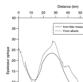
Ž .
Fig. 8. Comparison of the optical depth retrieved from lidar measurements at 532 nm and from the cloud albedo analysis using ARAT flux measurements for leg MA2.
comparable between the two. In the optically denser part of the cloud, values are in good
Ž .
agreement about 20% or better . On the other hand, CODs retrieved from passive measurements are larger in the other parts of the cloud. Most likely, this discrepancy is due to a combination of effects: cloud inhomogeneity and the fact that the lidar and the pyranometers have different fields of view. It could also be related to the simplified
Ž Ž ..
COD calculation used i.e. Eq. 6 . This point will be further investigated.
5. Retrieval of cloud microphysics
Ž .
above the cloud base Brenguier, 1991 . The cloud extinction coefficient a, is defined as the extinction cross-section averaged over the whole droplet size distribution
`
2
a
Ž
z ,l.
spH
QeŽ
r ,l.
r N r d r ,Ž .
Ž .
70
where Q is the extinction efficiency. From Mie theory calculations, this factor dependse on the size parameter xs2prrl, which is a function of droplet radius r but also of wavelength l. Q is maximal for xe s6 at visible wavelengths. At x values larger than
10, the extinction efficiency decreases to the asymptotic value Qes2, with damped
Ž .
oscillations see for example Pinnick et al., 1983 . Assuming the droplet distributions in the sampled clouds under study have a modal radius larger than a few microns, we can
consider that at the measurement wavelength ls532 nm, Q can be approximated bye
Ž .
an analytical expression Pinnick et al, 1983 ,
Q
Ž .
x s2 1Ž
qxy2r3.
,Ž .
8e
and calculated for the value of x corresponding to the mode radius of the distribution.
Q varies between 2.23 and 2.08 for mean droplet radius ranging between 2 and 10e mm.
This range encompasses most of the cases of droplet distributions in warm clouds
ŽBower et al., 1994 , assuming a factor 0.6 between the mean and effective radius, as.
estimated from a gamma droplet size distribution.
Ž .
The extinction coefficient a given by Eq. 7 is thus proportional to the second order moment of the droplet size distribution. Neglecting high order fluctuations, assumed to be of second order at the measurement scale,a can be simply written as the ratio of the
Ž .
liquid water content and the effective radius Pinnick et al., 1983 . In the case of an adiabatic increase of liquid water content with height, the effective radius at cloud top
Ž .
As the value of Q depends on the average droplet radius, a correction may be appliede
Ž . Ž .
using Eq. 8 . However, this correction remains small less than 5% and in this paper,
we have used the average value Qes2.16, close to the value Qes2.2, obtained by
PBB. Should drizzle occur near cloud top, the extinction coefficient can be written as the sum of two independent contributions: extinction due to cloud droplets and to drizzle as there is no overlapping between their size distributions. The drizzle liquid water content being smaller than the cloud one, and the effective radius of drizzle being more than 10 times larger than the droplet one, the extinction coefficient is mainly sensitive to the cloud droplet contribution.
Ž
The temperature at cloud base height zb being close to 28C as obtained from
.
soundings , the coefficient Cw defining the adiabatic increase of liquid water is equal to
y3 y4 Ž . )
1.5 10 g m Brenguier, 1991 . The maximum cloud geometrical depth is zt s520
Ž . y1
m Fig. 3 and the maximum extinction coefficient at the cloud top is about 0.17 m
ŽFig. 6 . Thus, we obtain r. es7.3mm at cloud top in the strongest updraft. The error is estimated to be about 15% from results plotted in Fig. 6, and from the approximation in
( ) J. Pelon et al.rAtmospheric Research 55 2000 47–64
62
effective radius is weakly varying close to cloud top, extinction fluctuations at cloud top reported in Figs. 5 and 6 can be mostly attributed to variations in liquid water content.
Ž ).
Following PBB, the droplet concentration N zt at cloud top is
3 2 3
Kat 1 16 Kr at
)
N z
Ž
t.
spQ rŽ
z).
s 9 pC z2 )2 Q ,Ž
10.
e e t w t e
where K is a size parameter depending on the ratio of the volume to effective radius
Žsee Martin et al., 1994 and PBB for more details taken equal to 0.8 for marine.
stratocumulus, and r is the liquid water density taken equal to 106 g my3. Using Eq.
Ž10 , the number of droplets deduced from lidar measurements in updrafts at cloud top is.
Ž ). y3
about N zt s390 cm , meaning that a fairly large number of nuclei have been
activated. This value is also in good agreement with in situ measurements of PBB.
Ž . Ž . Ž ).
According to Eq. 10 , uncertainties are large )30% because N zt is proportional to
the third power of the extinction coefficient at the cloud top.
The vertical distribution of the cloud droplet concentration can be considered, to the
Ž Ž ). Ž ). . Ž ).
first order, as constant with height N z sN zt , see PBB . However, N z
depends on the horizontal location in the cloud, and differences may be observed
Ž .
between updrafts and downdrafts. From Eq. 10 and cloud droplet concentration
obtained at cloud top, the vertical profile of the extinction coefficient in an adiabatic updraft is given as a first approximation by the expression
2r3
) y3
w
)x
a
Ž
z.
s2.87=10 z ,Ž
11.
) Ž .
where z is in meters and a is in inverse meters. The adiabatic limit given by Eq. 11
Ž . Ž y3.
has been plotted on Fig. 6. Recall that the coefficient in Eq. 11 i.e. 2.87=10 is
calculated using the largest lidar-derived extinction value and cloud thickness value
Ž . Ž .
observed i.e. for the strongest updraft observed by lidar . Eq. 11 should provide an estimate of the maximum extinction coefficient to be expected as a function of altitude. The fact that most of the observations are found systematically to the left of the dotted
Ž
curve instead of falling on the curve as expected if the increase in liquid water was
.
adiabatic is consistent with the fact that, in Fig. 6, we have not selected data from updrafts only and is compatible with the uncertainty related to the lidar-derived extinctions.
Ž .
Inversely, the theoretical limit provided by Eq. 11 can be used to define the cloud
Ž .
geometrical thickness or cloud base altitude, indifferently , if the cloud top altitude,
Ž
droplet concentration and adiabatic liquid water content are known as was done in Fig.
.
6 . This inverse approach can be of interest in the context of space-borne studies. A scatter plot, such as the one shown in Fig. 6, can be used to retrieve a first guess for the
Ž . Ž .
altitude of the extinction at the top of the most energetic updraft s .
6. Conclusion
depth values larger than 10 have been retrieved. Due to the high spatial resolution of lidar measurements, convective cells within the stratocumulus deck can be evidenced from cloud top height increase. Large values of the lidar-derived extinction coefficient at cloud top have been observed to be associated to convective cells. In such cells, the estimated optical depth reached values close to 40, which agreed within 10% with the values calculated under the adiabatic hypothesis. Average values of the COD are in good agreement with values derived from albedo analysis. In convective cells, the effective radius and droplet concentration were also shown to be in good agreement with in situ measurements. These values of the cloud parameters will also be compared to other estimates derived from radiometer measurements in the conclusion paper of the series
ŽPawlowska et al., 2000b . The results are encouraging and the method will be refined.
for the analysis of other stratocumulus cloud cases. It could be further applied to the retrieval of cloud properties from space if cloud geometrical thickness can be deter-mined remotely. In case of broken stratocumulus, the determination of this parameter at the mesoscale is possible using lidar data only. In other cases, theoretical limit provided
Ž .
by Eq. 11 could be used to estimate the cloud base height, assuming a standard value
Ž
of the number of droplets depending on the observed cloud type maritime or
continen-.
tal , as discussed in Section 5. A scatter plot, such as the one shown in Fig. 6, can be
Ž .
used to retrieve a first guess for the altitude of the extinction at the top of the most
Ž .
energetic updraft s . This information, combined with the knowledge of the number of cloud droplets, can be used to infer the proportionality coefficient between z) and a,
and, in turn, the altitude of the cloud base.
Acknowledgements
Financial support for the ARAT flights and for the study which was received from
Ž .
the EC Environmental and Climate Division under grant EV5V-CT 92-0130 , and from
the Programme Atmosphere et Ocean a Moyenne Echelle of INSU-CNRS are acknowl-
`
´
`
edged. ARAT data would not have been acquired and processed without the support of the INSUrDT aircraft team and the help of IGN pilots to whom the authors are grateful.
References
Boucher, O., Lohman, U., 1995. The sulfate-CNN-cloud albedo effect: a sensitivity study using two general circulation models. Tellus 47, 281–300.
Bower, K.N., Choularton, T.W., Latham, J., Nelson, J., Baker, M.B., Jensen, J., 1994. A parameterization of
Ž .
warm clouds for use in atmospheric general circulation models. J. Atmos. Sci. 51 19 , 2722–2732. Brenguier, J.-L., 1991. Parametrization of the condensation process: a theoretical approach. J. Atmos. Sci. 48,
264–282.
Brenguier, J.L., Fouquart, Y., 2000. Introduction to the EUCREX-94 mission 206. J. Atmos. Res., this issue. Cahalan, R.F., Ridgway, W., Wiscombe, W.J., Bell, T.L., 1994. The albedo of fractal stratocumulus. J. Atmos.
Ž .
Sci. 51 16 , 2434–2455.
( ) J. Pelon et al.rAtmospheric Research 55 2000 47–64
64
Chepfer, H., Brogniez, G., Sauvage, L., Flamant, P.H., Trouillet, V., Pelon, J., 1999. Remote sensing of cirrus radiative properties during EUCREX ’94. Case study of 17 April 1994: Part 2. Microphysical modelling. Mon. Weather Rev. 127, 504–518.
Doutriaux, M., Pelon, J., Trouillet, V., Seze, G., Le Treut, H., Flamant, P.H., Desbois, M., 1998. Simulation of the Cloud climatology observed from space by a backscatter lidar and radiometers using the LMD General Circulation Model. J. Geophys. Res. 103, 26,025–26,039.
Flamant, C., Pelon, J., 1996. Atmospheric boundary layer structure over the Mediterranean during a Tramontane event. Q. J. R. Meteorol. Soc. 122, 1741–1778.
Flamant, C., Trouillet, Chazette, P., Pelon, J., 1998. Wind speed dependence of atmospheric boundary layer optical properties and ocean surface reflectance as observed by airborne backscatter lidar. J. Geophys. Res. 103, 25,137–25,158.
Flamant, P.H., Elouragini, S., Pelon, J., 1996. Etude preliminaire de la mesure simultanee par lidar du rayon´ ´
Ž .
effectif des gouttelettes et du contenu en eau nuageuse. C.R. Acad. Sci. Paris 323 serie II a , 563–568.´
Fouquart, Y., Buriez, J.C., Herman, M., Kandel, R., 1990. The influence of clouds on radiation: a climate modeling perspective. Rev. Geophys. 28, 145–166.
Fouilloux, A., Gayet, J.-F., Kriebel, K.-T., 2000. Determination of cloud microphysical properties from AVHRR images: comparison of three approaches. J. Atmos. Res., this issue.
Kiehl, J.T., 1994. Sensitivity of a GCM climate simulation to differences in continental versus maritime cloud drop size. J. Geophys. Res. 99, 23,107–23,115.
Martin, G.M., Johnson, D.W., Spice, A., 1994. The measurement and parametrization of effective radius of droplets in warm stratocumulus clouds. J. Atmos. Sci. 51, 1823–1842.
Meador, W.E., Weaver, W.R., 1980. Two-stream approximations to radiative transfer in planetary atmo-spheres: a unified description of existing methods and a new improvement. J. Atmos. Sci. 37, 630–643. Pawlowska, H., Burnet, L., 2000a. Microphysical properties of stratocumulus clouds. J. Atmos. Res., this
issue.
Pawlowska, H., Brenguier, J.L., Fouquart, Y., Armbruster, W., Descloitres, J., Fischer, J., Flamant, C., Fouilloux, A., Gayet, J.F., Ghosh, S., Jonas, P., Parol, F., Pelon, J., Schuller, L., 2000b. Microphysical and¨
radiative properties of stratocumulus cloud: the EUCREX mission 206 case study. Atmos. Res., this issue. Pinnick, R.G., Jennings, S.G., Chyleck, P., Ham, C., Grandy, W.T., 1983. Backscatter and extinction in water
clouds. J. Geophys. Res. 88, 6787–6796.
Platt, C.M.R., 1973. Lidar and radiometric observations of cirrus clouds. J. Atmos. Sci. 30, 1191–1294. Raschke, E., Flamant, P.H., Fouquart, Y., Hignett, P., Isaka, H., Jonas, P.R., Sundquist, H., Wendling, P.,
Ž .
1997. Cloud-radiation studies during the European cloud and radiation experiment EUCREX . Surv. Geophys.
Saunders, R.W., Brogniez, G., Buriez, J.C., Meerkotter, R., Wendling, P., 1992. A comparison of measured¨
and modeled broadband fluxes from aircraft data during the ICE ’89 filed experiment. J. Atmos. Ocean. Technol. 9, 391–406.
Sauvage, L., Chepfer, H., Trouillet, V., Flamant, P.H., Brogniez, G., Pelon, J., Albers, F., 1999. Remote sensing of cirrus radiative properties during EUCREX ’94. Case Study of 17 April 1994: Part 1. Observations. Mon. Weather Rev. 127, 486–503.
Spinhirne, J.D., Boers, R., Hart, W., 1989. Cloud top liquid water from lidar observations of marine stratocumulus. J. Appl. Meteorol. 28, 81–90.
Trouillet, V., 1997. Etude de l’apport d’un lidar retrodiffusion spatial pour la retsitution des parametre nuageux´ `
Ž . w
et de flux a la surface. PhD dissertation Universite Pierre et Marie Curie, Paris, France , 289 pp Available` ´
from Service d’Aeronomie du CNRS, Universite Pierre et Marie Curie, 4 place Jussieu, 75252 Paris Cedex´ ´
x 05, France .
Twomey, S., 1977. The influence of pollution on shortwave albedo of clouds. J. Atmos. Sci. 34, 1149–1152. Valentin, R., Flamant, C., Flamant, P., Pelon, J., Spinhirne, J., Hart, W., 1994. Lidar observations of marine stratocumulus during ASTEX. 2nd International Conference on Air–Sea Interaction and on Meteorology, Lisbonne.