The New Approach to Camera Calibration
–
GCPs or TLS Data?
J. Markiewicza,* P. Podlasiaka, M. Kowalczyka, D. Zawieskaa
a
Faculty of Geodesy and Cartography, Department of Photogrammetry, Remote Sensing and Spatial Information Systems, Warsaw University of Technology, Warsaw, Poland – (j.markiewicz, p.podlasiak, m.kowalczyk, d.zawieska)@gik.pw.edu.pl
Commission WG III/1
KEY WORDS: Calibration, OpenCV, BLOB Detectors, Corner Detectors, TLS calibration field
ABSTRACT:
Camera calibration is one of the basic photogrammetric tasks responsible for the quality of processed products. The majority of calibration is performed with a specially designed test field or during the self-calibration process. The research presented in this paper aims to answer the question of whether it is necessary to use control points designed in the standard way for determination of camera interior orientation parameters. Data from close-range laser scanning can be used as an alternative. The experiments shown in this work demonstrate the potential of laser measurements, since the number of points that may be involved in the calculation is much larger than that of commonly used ground control points. The problem which still exists is the correct and automatic identification of object details in the image, taken with a tested camera, as well as in the data set registered with the laser scanner.
1. INTRODUCTION
Together with the continuing growth in demand for precise measurement technologies observed nowadays, close-range photogrammetric methods based on non-metric cameras compete with other measurement technologies. Non-metric cameras offer sophisticated functions such as autofocus, zoom lenses or image stabilization, which limit their measuring potential. Therefore, to use non-metric cameras in photogrammetric applications, the appropriate camera calibration method should be used. Camera calibration has always been a crucial part of photogrammetric measurements. The exact determination of internal camera orientation parameters is a condition for obtaining precise and reliable information from the images. Therefore, the current issue in close-range photogrammetry is the study of calibration techniques during research into the practical possibilities of the utilization of non-metric digital cameras. Nowadays, self-calibration is an integral part of measurements which are commonly used in close-range photogrammetry and ComputerVision methods based on Structure from Motion (SFM) algorithms. This method has many advantages, but requires an adequate image network, which cannot always be achieved. Therefore, non-metric camera calibration based on point cloud registered with TLS technology can be an alternative to the special test fields used for calibrating cameras. The aim of this paper is to perform experiments which will verify the thesis assumed by the authors that non-metric cameras can be calibrated based on TLS data. Such a process is often required when it is necessary to use images taken at a different time from the scans, and the calibration data of the camera used for taking these images do not exist.
The authors have created the C++ application which uses free OpenCV and Lappac libraries and can be used for single image calibration. For photogrammetric control point extraction on the images and the TLS scan, different corner and BLOB detectors are used and the different descriptions generated by the respective descriptors are utilized to combine them. Such an approach allows the elimination of the creation of a special test field; hence the calibration process can be performed in the
field. Thanks to the utilization of automatically determined natural points, the number of control points is increased and they are evenly distributed. As the result of experiments performed it was proven that the calibration process ran smoothly when the point cloud was transformed to the raster form. The least square method and procedures implemented in the OpenCV suite were used for interior and exterior orientation parameters determination.
This paper presents the comparison of results of camera calibration performed in the classic way and with the use of the method proposed by the authors. Additionally, it shows the photogrammetric products obtained with the use of calibration results, confirming its correctness.
2. RELATED WORK IN CAMERA CALIBRATION
The market introduction of inexpensive cameras with less stable lenses made it necessary to perform calibration at the time of object registration, due to the possible time-changes of camera parameters. Since the research works on camera field calibration performed by Heller and Brown and Brown’s implementation of the independent rays bundle adjustment in 1968, there have been several possibilities for field calibration of close-range cameras (Clarke and Fryer, 1998). These methods are mainly based on taking pictures of test fields and their classification depends on test types, the geometrical conditions of image registration, methods of calculations and the required accuracy. There are several criteria for classification. In order to include the collinearity condition in the calibration process, two basic functional models – the perspective and the projective model – are used (Remondino and Fraser, 2006).
Calibration performed independently from registration of an analysed object can be performed by analysis of one image or a group of images. If a single image is used, its field of view must contain a set of correctly marked points of known 3D co-ordinates, not localized on a common plane. The larger the number of points and their spatial differentiation, the more reliable the calibration results. The greater number of simultaneously processed images corrects the results, since the degree of correlation between individually calculated parameters of interior as well as exterior orientation decreases. The case of use of several images makes it possible to reduce the form of the test-field used for full calibration to a flat board. Recently, the methods based on the analysis of distribution of straight lines or parallel curves of specific directions in the image (Wang et al., 2007), have become more popular, being methods which do not require a specially prepared test field. Instead, they use in-the-field calibration based on the geometrical relationships in the object space. The knowledge of the spatial points is not necessary in such methods, as the calculation of interior orientation parameters is based on the conditions of orthogonality and coplanarity. If the approximate values of external camera orientation parameters are given, the calculation is performed as a result of hybrid independent rays bundle adjustment. If we have no such information, the alternative method can be used based on the condition of orthogonality and coplanarity of two parallel section pairs in object space. These sections should be the longest and most convergent in the picture. In order to determine the position of the principal point and the focal length, six pairs of parallel vectors should be defined in such a way that each pair would be perpendicular to each other in the space. They may be visible in different images taken with the same focal length (Kraus, 1997; Ohdake, Chikatsu, 2007).
The term ―self-calibration‖ is understood as calculation of the interior orientation parameters, which takes place during the adjustment process including the calculation of the object point co-ordinates and external camera orientation parameters. This method is the most effective for digital images (Kraus, 1997; Clarke and Fryer, 1998; Cardenal et al., 2004); however, it requires a set of images of different geometry. Currently, many different approaches to create a model describing the projection performed by the camera are used worldwide. Depending on the selected calibration mode,
different sets of parameters are used. For many years, Brown’s
model has been the most popular; it was created in the 1950s and later described in analytical form (Brown, 1971). It includes three parameters of camera interior orientation, called IO (Interior Orientation). These include an image distance, also called a camera-fix, and the co-ordinates of the main point of autocollimation, which is a projection of the projection centre on the camera image plane.
Other parameters are the coefficients describing the radial and tangential distortion, which present the distribution of the
projection’s systematic errors, carried on a camera image plane.
The number of images available in the calculation requires the use of specific procedures for parameter definition (Tang, 2013). These procedures vary depending on the type of camera used for measurements. The camera with a narrow, a normal and a wide-angle lens, including a camera equipped with a fisheye lens, requires a different approach (Frank et al., 2006). Generalizing information about calibration measurements, it can be assumed that the greater the number of observations existing in the data set, the better the opportunity to determine the projection realized by the camera. The greater number
of pictures can be replaced by a larger number of observations present in a single image. These observations should be represented by the knowledge of the three-dimensional shape of the photographed object and adopted as a measurement test.
2.1 The photogrammetric approach vs. CV
The classic photogrammetric approach to camera calibration is based on the assumption of collinearity of three points: in the 3D space (X, Y, Z), its image in the photograph (x, y) and the Any errors caused by distortion, etc. are corrected in accordance
with Brown’s model (Brown, 1971).
In ComputerVision these relationships are described with the use of homogeneous coordinates: describing simultaneously interior and exterior orientation.
Distortions are described with the same Brown’s model but the
values and the number of coefficients are different (the OpenCV model allows for the appointment of one to six radial distortion coefficients – which stems from the use of non-metric cameras). During the calibration process using procedures of OpenCV suite (calibrateCamera procedure), the projection matrix is calculated, which is then separated into the camera matrix (M1 interior orientation) and exterior orientation matrix (M2). A detailed comparison of the estimated parameters can be found in the literature (Wang, 2012; Zhang, 2008).
3. THE NEW CONCEPT OF CAMERA CALIBRATION
The process of automatic calibration of close-range images with the use of terrestrial laser scanning data has been performed with the use of the processed Target-based registration method expanded with Feature-Based point detection.
The top algorithms used in CV were used in experiments. The authors’ approach in the calibration process was to use natural points in scan In the proposed algorithm, raster images from scans in the form of orthoimages (supplemented with the depth map) were generated at first. Then, in order to automatically search for corresponding natural points in the images and orthoimages (intensity and shaded DSM), the algorithms based on corner detection were used:
BRISK (Leutenegeer et al., 2011),
FAST (Rostem, 2006) and BLOB algorithms:
MSER (Matas et al., 2002),
SIFT (Lowe, 2004),
The co-ordinates of detected points were processed from the 2D form into 3D co-ordinates by knowing the co-ordinates X, Z in the orthoimage; the Y value was taken from the depth map. It was then possible to analyse the use of automatically identified natural points for calibration. In order to objectively assess the authors’ approach to camera calibration:
the number and distribution of points in images and orthoimages was tested,
the percentage of correctly detected and matched key-points was analysed,
the calibration accuracy of algorithms used in the photogrammetric approach and in CV was analysed,
the accuracy and correctness of calibration using the points (GCPs) detected automatically and manually were analysed,
the accuracy of orthoimages generated with the use of images with removed distortion and shifted principal point was analysed.
3.1 The data used
For analyses, the point clouds registered with the terrestrial laser scanner Z+F 5003 of a part of a facade of the Museum of King
Jan III’s Palace at Wilanów and close-range images taken with the Nikon D3X equipped with two 50mm lenses and a zoom lens of 28-135 mm were used. The point clouds were registered with the resolution of 3mm/10m. The maximum distance from the station was 30m and the minimum distance was 3m. The acquired data were initially filtered by the reflectance intensity.
3.2 TLS data processing
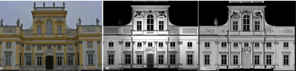
The spherical images generated as the result of point cloud processing are characterized by large distortions similar to the distortion effect occurring on digital images. Unfortunately, the part of detected tie points is not correctly matched by the descriptors (Markiewicz, Markiewicz, 2015). The solution to this problem may be the transformation of the point cloud into the form of an orthoimage. In order to do this, the approach proposed by the authors was used (A New Approach to the Generation of Orthoimages of Cultural Heritage Objects -Integrating TLS and Image Data (Markiewicz et al., 2015). This process was performed in a fully automatic way. First, the reference plane was detected with the use of the processed Hough algorithm. The point cloud was then projected onto the a specified plane. In order to fill the occluded areas on the resulting orthoimage, the nearest neighbour interpolation method was used (Fig. 1). Additionally, the depth map was saved.
3.3 Key-points searching and matching
In the first step, the point-detecting algorithms in RGB images and in shaded DSM in the form of an orthoimage were tested. As default parameters the values proposed by the authors of the mentioned algorithms were used. The SIFT descriptor was chosen as the descriptor for all methods (as per the literature). Part of the points was identified and matched incorrectly. This was caused by the different spectrum of an electromagnetic wave registered by the scanner and registered in the images. The process of elimination of outliers was performed iteratively:
Eight points were measured manually in the scan and the image.
The approximate parameters’ values were appointed for
3D DLT transformation. The advantage of this transformation is the fact that initial interior orientation parameters are not required.
Such points were removed for which the differences between theoretical image co-ordinates calculated on the basis of the 3D DLT transformation parameters and the co-ordinates detected by the algorithms were greater than 50 pixels.
In order to assess the suitability of the use of different algorithms, the number of points detected, the number of correctly detected points (Tab. 1) and the distribution of points (Figs. 2 and 3) were evaluated. The correctness of tie point detection was also tested depending on the distortion influence. The second image analysed was the image with the high distortion values (an image taken with zoom lens with unknown focal length). As in the previous case, the same detectors and descriptors for the detection of tie points used in the calibration process were used.
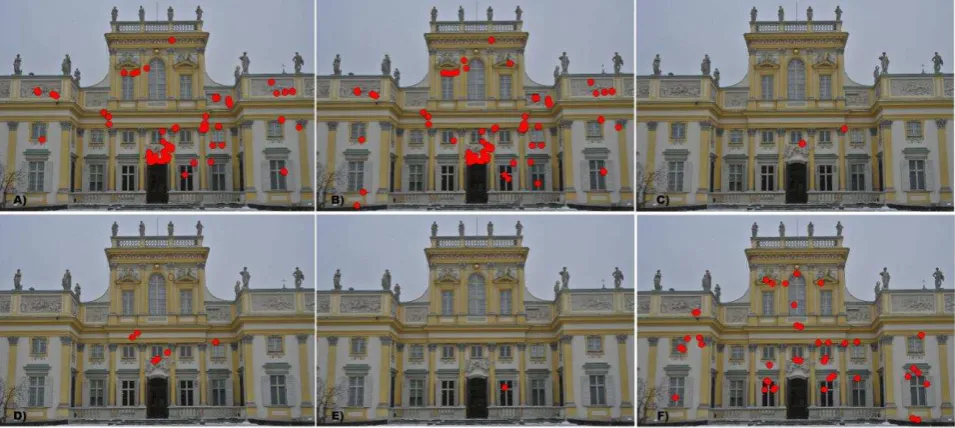
Analysing Table 1, a considerable decrease in the number of points can be noticed, compared with the number of points detected in the less distorted image. As in the previous case (the less distorted image), the same dependence can be noticed between the detector type and the number of points detected in the orthoimages of a different type. Additionally, the influence of detector selection for the tie point distribution in the image was tested. Figure 2 presents the distribution of points detected for A) BRISK, B) FAST, C) STAR, D) MSER, E) SIFT and F) SURF detectors, respectively.
Fixed lens Zoom lens Intensity orthoimage Shaded DSM transformed
to the image form Intensity orthoimage
Shaded DSM transformed to the image form Number
of points
Number of correctly detected points
Number of points
Number of correctly detected points
Number of points
Number of correctly detected points
Number of points
Number of correctly detected points
BRISK 530 5 530 40 32 1 14 1
FAST 3,055 137 4,476 158 576 74 246 78
STAR 235 3 320 3 40 0 14 2
MSER 65 11 17 7 204 31 101 16
SIFT 106 4 85 1 34 1 12 0
SURF 975 108 612 44 293 69 117 13
Table 1. The number of points detected on two images by different algorithms.
Figure 2. The distribution schema of points detected in the image and in the intensity image for A) BRISK, B) FAST, C) STAR, D) MSER, E) SIFT and F) SURF detectors, respectively.
Analysing the schemas shown in Figure 2, it can be noticed that by far the best distribution of points was obtained when using the BRISK, FAST and MSER algorithms. Unfortunately, the use of only one detector does not provide satisfactory results. A similar analysis was performed for points detected on the shading orthoimage. Figure 3 presents the distribution of points detected on the shaded DSM transformed into the image form for A) BRISK, B) FAST, C) STAR, D) MSER, E) SIFT and F) SURF detectors, respectively.
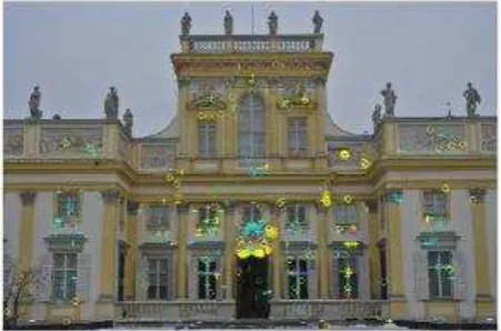
In order to obtain the correctly distributed points in the calibrated image, several algorithms of point detection and image matching must be combined and homologous points should be detected in the intensity orthoimage and the shaded DSM stored in the form of orthoimages (Fig. 4).
Figure 4. One of the images with superimposed points used in the calibration process.
3.4 The calibration process
The evaluation of correctness of the geometrical camera parameter calculation was performed by comparing results resulting from two approaches. On the one hand, close-range laser scanning was used in the standard single image calibration. Comparative results were provided by the self-calibration performed on the series of images.
3.4.1 Self-calibration
The self-calibration process was performed with the use of Agisoft PhotoScan software. Four images acquired with a Nikon D3X camera (full-frame camera) equipped with a 50mm lens and four images acquired with a Hasselblad H4D-50 (middle-frame camera) equipped with an 80mm lens were used. The obtained camera model described is similar to that in
Brown’s description (Brown, 1971). In order to convert the
co-ordinates of the principal point, the image co-ordinate system was assumed in the centre of the tested image. This resulted in the necessity to transform the system implemented in Agisoft, the origin of which is located in the upper left corner.
3.4.2 Single image calibration
Calculation of the camera calibration parameters was performed based on one of the images used for self-calibration. As the control points for manual measurement, 24 evenly distributed points (GCPs) were used; they were measured with the Z+F
5006h scanner. Calculations were made with the use of ―Kalib‖
software performing the classic parametrical model for the camera description (Brown, 1971). Table 2 presents the values
of camera calibration parameters obtained from self-calibration and calculation based on a single image.
The comparison also applies for determining the characteristics of projection errors. It was decided to describe them using the first three radial distortion parameters. Figure 5 presents the course of the tested error of derogation from the central projection implementation by the camera. The presented values and the function arguments are expressed in pixels.
Method \ Parameter x0 (pix) y0 (pix) ck (pix) Self-calibration -48.96 37.73 8,703.50 Single image calibration -24.47 5.18 8,724.83 Table 2. The comparison of camera interior orientation elements calculation results performed with two methods.
Figure 5. Comparison of distortion values for both methods of calculation. Red – self-calibration with Agisoft (parameters k1, k2, k3 of radial distortion); Green – single image calibration (parameters k1, k2, k3 of radial distortion).
The results show the greater value of distortion error calculated based on a single image along the radial radius in the range from 500 to 2,700 pixels.
3.4.3 Calibration with points found on scans and the ComputerVision method
The approach conducted using the algorithms used in the machine vision uses points automatically detected in photographs and orthoimages in intensity and shaded DSM. By using algorithms implemented in OpenCV it was possible to select various parameters describing the radial distortion. In the adopted calibration method calibrated focal length was divided into the x and y components. In this research the calibration was performed using the radial distortion parameter: k1 only and all three parameters k1, k2 and k3.
In addition, in order to examine the validity of the use of CV algorithms, the calibration performed using designed GCPs was tested.
3.5 Analysis of results and discussion
The results of calibration performed with the use of three different techniques have been analysed. The relationships were tested between the value of the calibrated focal length and the adopted calibration method. Unfortunately, due to the fact that each of the tested algorithms describes the distortion in a different way, it was only possible to evaluate the distortion depending on the distance from the principal point. This evaluation was made with the use of charts presented earlier in this article.
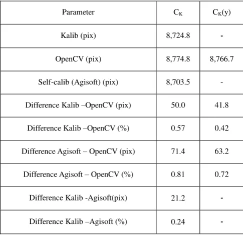
Difference Kalib –OpenCV (%) 0.57 0.42
Difference Agisoft – OpenCV (pix) 71.4 63.2
Difference Agisoft – OpenCV (%) 0.81 0.72
Difference Kalib -Agisoft(pix) 21.2 -
Difference Kalib –Agisoft (%) 0.24 -
Table 3. The calibrated focal length values, differences between methods and percentage value of differences for the fixed lens. Analysing Table 3, it can be noticed that all these methods allow the achievement of similar values for the calibrated focal length. The differences between them do not exceed 75 pixels and, referring to the average focal length, do not exceed 1%. This may suggest that, in the case of the proposed method, the accuracy of determination of the camera constant value (ck) is comparable with values obtained using calibration with a designed calibration test field. Analysing the graphs of distribution of the radial distortion values, some convergences between them can be noticed (Figs. 5 and 6). Similar tests were performed for the zoom lens camera. The focal length value was unknown; it was set so that the subject fully filled the entire frame.
Parameter Kalib zoom lens, the proposed calibration method not based on GCPs designed earlier allows the correct camera calibration to be performed.
4. GEOMETRIC EVALUATION OF THE PROCESSED ORTHOIMAGES
In order to perform an independent accuracy assessment of the influence of the obtained calibration parameters on the accuracy of the final photogrammetric products, orthoimages such as RGB and Intensity were analysed. The basic assumption of the adopted camera calibration method was the correction of only a selected fragment of the image (i.e., the so-called zonal calibration). Fragments of images corrected this way and connected together created the entire RGB orthoimage. The resulting orthoimage was characterized by higher quality due to the earlier removal of distortions in fragments of the entire study area.
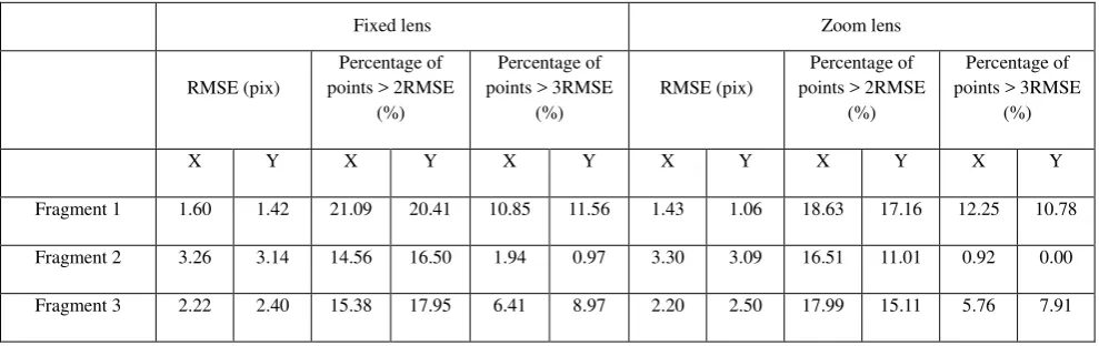
In order to determine the quality of the final products, the geometrical quality of fragments of RGB orthoimages was tested. For this purpose, we examined the geometric quality of points detected by the SURF detector and matched with the SURF detector in the intensity and RGB orthoimages.
In the proposed control method, the co-ordinates were fragments where the higher number of tie points was found, the considerably higher accuracy can be noticed (Fragments 1 and 3), the lower value of RMSE of differences between points can be seen, not exceeding 2.5 pixel. In the case of Fragment 2 the values of RMSE slightly exceeded 3 pixels.
Figure 7. The scheme of test field localization used for camera calibration accuracy analysis. orthorectification process. Despite this, the results obtained are consistent and allow the conclusion to be drawn that the proposed method of automatic calibration based on the TLS data can (and should) replace the classic approach based on the field calibration using points (GCPs).
Fixed lens Zoom lens
RMSE (pix)
Percentage of points > 2RMSE
(%)
Percentage of points > 3RMSE
(%)
RMSE (pix)
Percentage of points > 2RMSE
(%)
Percentage of points > 3RMSE
(%)
X Y X Y X Y X Y X Y X Y
Fragment 1 1.60 1.42 21.09 20.41 10.85 11.56 1.43 1.06 18.63 17.16 12.25 10.78
Fragment 2 3.26 3.14 14.56 16.50 1.94 0.97 3.30 3.09 16.51 11.01 0.92 0.00
Fragment 3 2.22 2.40 15.38 17.95 6.41 8.97 2.20 2.50 17.99 15.11 5.76 7.91
Table 5. The error values and the percentage of points greater than 2RMSE and 3RMSE for calibration with the ComputerVision method.
Fixed lens Zoom lens
RMSE (pix)
Percentage of points > 2RMSE
(%)
Percentage of points > 3RMSE
(%)
RMSE (pix)
Percentage of points > 2RMSE
(%)
Percentage of points > 3RMSE
(%)
X Y X Y X Y X Y X Y X Y
Fragment 1 1.31 1.20 19.59 20.62 11.34 11.86 1.37 1.24 19.88 19.88 12.65 11.44
Fragment 2 3.17 3.59 18.92 10.81 1.31 2.70 2.75 2.98 14.14 16.16 4.04 2.02
Fragment 3 2.51 2.80 17.31 20.19 6.73 5.80 2.44 2.54 13.27 20.35 7.96 5.31
Table 6. The error values and the percentage of points greater than 2RMSE and 3RMSE for calibration with the photogrammetric method.
Fixed lens Zoom lens RMSE (pix) RMSE (pix)
X Y X Y
Fragment 1 0.29 0.22 0.06 -0.18 Fragment 2 0.09 -0.45 0.55 0.11 Fragment 3 -0.29 -0.4 -0.24 -0.04
Table 7. The error differences between calibration performed with GCP and TLS data.
5. CONCLUSIONS
The research performed resulted in a number of practical tips for camera calibration without the necessity to use a test field. It may be replaced by TLS data. The algorithms used in the CV largely automate the camera calibration process. After the conversion of TLS data to the raster form, better results of homologous points are accomplished using a line detectors on the shaded DSM. When using BLOB detectors, it is recommended to use the intensity orthoimages.
In the case in which the algorithms from the OpenCV library are used, it is possible to use different radial distortion coefficients but it is necessary to give the approximate focal length value, even with low accuracy. In the calculation process the fast convergence of the solution is an advantage,
even in the presence of gross errors. The results indicate significant potential of the presented approach in the practice of measurements. The camera parameters calculated with the use of this method (hence with the use of point cloud obtained from terrestrial laser scanning) show considerable similarity to results from the self-calibration method. Therefore, it is possible to use test fields acquired up to date in the field to calibrate the cameras used to create the architectural inventory documentation. This is particularly important when the scans and the images are acquired at different times and camera calibration is not performed. This is especially useful when the high-resolution orthoimages of cultural heritage are processed where scans and images are acquired independently.
REFERENCES
Brown D.C., 1968, Anvanced Methods for The Calibration of Metric Cameras, U.S. Army Engineer Topographic Laboratories, Fort Belvoir, Virginia 22060.
Brown D.C. 1971, Close-Range Camera. Calibration. Photometric Engineering. vol. 37. no. 8, pp. 855-866. Cardenal J., Mata E., Castro P., Delgado J., Hernandez M. A.,
Prerez J. L., Ramos M., Torres M., 2004, ―Evaluation
of a digital non metric camera (Canon D30) for the
photogrammetric recording of historical buildings‖,
Clarke T.A., Fryer J.G, 1998, ―The development of camera calibration methods and models‖, The Photogrammetirc
Record, 1998, Vol. 16(91), pp. 51-66.
Devernay F., Faugeras O., 2001, „ Straight lines have
to be straight. Automatic calibration and removal of distortion
from scenes of structured environments‖, Machine Vision
and Applications (2001) 13: 14-24.
Bay H., Tuytelaars T., Van Gool L., 2006, "SURF: Speeded Up Robust Features", Proceedings of the ninth European Conference on Computer Vision.
Frank A. van den Heuvel, Verwaal R., Beers B., 2006,
„Calibration of fisheye camera systems and the reduction of chromatic aberration―, ISPRS Commission V Symposium
Image Engineering and Vision Metrology.
Habrouk H.E., Li X.P., Faig W., 1996, „Determination
of Geometric Characteristics of a Digital Camera by
Self-Calibration‖, International Archives of Photogrammetry and
Remote Sensing, Vol.XXXI, Part B1.
Kraus K., 1997, „Photogrammetry Advanced Methods and Applications‖, Vol 2, Ferd. DummlerVerlag.
Leutenegger S., Chil M., Siegwart R. Y., 2011, " BRISK: Binary Robust invariant scalable keypoints." Proceeding ICCV '11 Proceedings of the 2011 International Conference on Computer Vision: 2548-2555.
Lowe D.G. 2004, "Distinctive Image Features from Scale-Invariant Keypoints". International Journal of Computer Vision 60 (2), pp. 91–110.
Markiewicz J., Podlasiak P., Zawieska D. 2015, "A New Approach to the Generation of Orthoimages of Cultural Heritage Objects—Integrating TLS and Image Data"., Remote Sensing, nr 7(12), pp. 16963-16985.
Markiewicz J., Markiewicz Ł. 2015, "Analysis of the algorithms for automatic spatial orientation of the clouds of points obtained with a terrestrial scanner". Informatics, Geoinformatics and Remote Sensing. Conference Proceedings V. I, Informatics, Geoinformatics, Photogrametry and Remote Sensing, International Multidisciplinary Scientific GeoConference & EXPO SGEM, vol. I, 2015, pp. 981-988.
Matas J., Chum O., Urban M., and Pajdla M., 2002, "Robust wide baseline stereo from maximally stable extremal regions." Proc. of British Machine Vision Conference, pp. 384-396.
McIntosh K., 1996, „A Calibration Procedure for CCD Array Cameras‖, International Archives of Photogrammetry and
Remote Sensing, Vol.XXXI, Part B1.
Remondino F., Fraser C, 2006, „Digital camera calibration methods: considerations and comparisons‖, ISPRS
Commission V Syposium Image Engineering and Vision Metrology.
Rosten E., 2006, "Machine learning for high-speed corner detection". Proceeding ECCV'06 Proceedings of the 9th European conference on Computer Vision - Volume Part I, pp. 430-443.
Ohdake, T., and Chikatsu H., 2007, Multi Image Fusion for Practical Image Based Integrated Measurement System, Optical 3D measurement Techniques VIII (1), pp. 56-63. Osgood T.J., Huang Y., 2013, Calibration of laser scanner and camera fusion system for intelligent vehicles using Nelder– Mead optimization, Measurement Science and Technology, 24.
Remondino F., Fraser C, 2006, „Digital camera calibration methods: considerations and comparisons‖, ISPRS
Commission V Syposium Image Engineering and Vision Metrology.
Tsai R.Y., 1987, "Metrology Using Off-the-Shelf TV Cameras and Lenses", IEEE Journal of Robotics and
Automation, Vol. 3, No. 4, pp. 323-344..
Wang H, Shen S. and Lu X., 2012, Comparison of the Camera Calibration between Photogrammetry and Computer Vision, International Conference on System Science and Engineering.