SELF-CALIBRATION OF TERRESTRIAL LASER SCANNERS: SELECTION OF THE
BEST GEOMETRIC ADDITIONAL PARAMETERS
J. L. Lerma*, D. García-San-Miguel
Photogrammetry & Laser Scanning Research Group (GIFLE). Department of Cartographic Engineering, Geodesy and Photogrammetry, Universitat Politècnica de València, Camino de Vera, s/n. 46022 Valencia, Spain – [email protected]
Commission V
KEY WORDS: LIDAR, Calibration, Geometric, Laser Scanning, Terrestrial, Accuracy
ABSTRACT:
Systematic errors are present in laser scanning system observations due to manufacturer imperfections, wearing over time, vibrations, changing environmental conditions and, last but not least, involuntary hits. To achieve maximum quality and rigorous measurements from terrestrial laser scanners, a least squares estimation of additional calibration parameters can be used to model the a priori unknown systematic errors and therefore improve output observations. The selection of the right set of additional parameters is not trivial and requires laborious statistical analysis. Based on this requirement, this article presents an approach to determine the best set of additional parameters which provides the best mathematical solution based on a dimensionless quality index. The best set of additional parameters is the one which provides the maximum quality index (i.e. minimum value) for the group of observables, exterior orientation parameters and reference points. Calibration performance is tested using both a phase shift continuous wave scanner, FARO PHOTON 880, and a pulse-based time-of-flight system, Leica HDS3000. The improvement achieved after the geometric calibration is 30% for the former and 70% for the latter.
* Corresponding author.
1. INTRODUCTION
Terrestrial laser scanning measurements are expected to be free of systematic errors by users and providers of this technology. Short details about accuracy are presented by manufacturers. The massive number of XYZ points with intensity values (and sometimes with colour) conceals the errors to non-experts in laser scanning. Errors in metric measurements are usually problematic not only for design and quality control but for modelling and reverse engineering especially in civil engineering, building construction and industrial applications.
Geometric calibration of terrestrial laser scanners, usually named self-calibration when it is carried out on-site, is normally approached from two perspectives, basically differentiated by the type of measured features. Furthermore, the feature usually sets the mathematical method. The methods based on planar features consider the equations of the planes while the target methods require a network of well-distributed spherical/planar targets (among others) from which their centroids are accurately determined. This paper will focus specifically on the second method making use of a reference network of target points. The reference network is realized by a set of target points accurately measured and subsequently adjusted. The differences between the laser scanning point clouds and the reference network will be used to model the error of the laser scanners.
The calibration of laser scanning systems is an active topic of research (Gielsdorf et al., 2004; Parian and Gruen, 2005, 2010; Lichti, 2007; 2009; 2010; Reshetyuk, 2009; Schneider, 2009; Reshetyuk, 2010; Soudarissanane et al., 2011; Glennie, 2012; Chow et al., 2013). The aim of the geometric calibration is to determine the optimal set of additional parameters which best describes the behaviour of the device itself. Once the required set of additional parameters are determined, the removal of the systematic errors is accomplished by applying these coefficients
to the observed measurements. This paper follows the mathematical model presented by Lichti (2007). A total of 21 calibration parameters (also called internal orientation parameters or additional parameters) can be considered, depending on the type of observable; up to 9 for the range, up to 7 for the horizontal angle and up to 5 for the elevation angle. Lichti (2007; 2009) for the FARO 880 suggests the complete error model, including not only the physical parameters but the empirical ones. Lichti et al. (2007) present an initial approach to the complete model in the evaluation of a Surphaser 25HS scanner.
Other researchers have developed self-calibration strategies basing the mathematical model on the use of planar observables. Gielsdorf et al. (2004) propose an adjustment based on planes to obtain a total station error model, calibrating a prototype device. Amiri Parian and Gruen (2005, 2010) extend the mathematical model of panoramic cameras to model the scanner’s sensor in the Imager 5003, but they only obtain the angular errors, not the range ones. Glennie and Lichti (2010) and Glennie (2012) present a simultaneous kinematic calibration and boresight adjustment of the Velodyne HDL-64E S2 laser scanning system considering planar features. Bae and Lichti (2007) raise the planar based self-calibration in order to remove the necessity of manually measuring the large number of targets. In their presentation, the on-site calibration method is proposed in order to repeat the calibration process in every measurement against a possible lack of stability of the parameters. Chow et al. (2011) validate the performance of point-based and plane-based self-calibration for the four most prominent errors in terrestrial laser scanners.
Various authors have centred their research on the study of the point-based method. In Kersten et al. (2005) a study of the MENSI GS100 is performed. The error in the distance measured and the trunnion axis error are analysed, by comparison with ISPRS Annals of the Photogrammetry, Remote Sensing and Spatial Information Sciences, Volume II-5, 2014
several distances taken by classical methods with the laser scanner. Kersten et al. (2005) associate a great part of the error to the properties of the surface features. Schneider (2009) proposes an alternative model (similar to Lichti (2008)) for the errors and evaluates it for a Riegl LMS-Z420i in two different test fields, and adding parameters stepwise to the model achieves two different parameterizations, one per each test field. González-Aguilera et al. (2009) check another error model (composed by 8 physical internal orientation parameters) on two pulse-based scanners: the Trimble GX200 and the Riegl LMS-Z390i, achieving significant precision and accuracy improvements for the former but not for the latter. García-San-Miguel and Lerma (2013) present an automatic strategy to carry out self-calibration of terrestrial laser scanning systems with local parameters instead of global parameters due to the instabilities of the FARO FOCUS 3D among scans under ideal conditions.
The laser scanning calibration performance usually yields several advantages far beyond the improvement in accuracy such as less noisy point clouds, lesser filtering needs and better mathematical estimations. The percentage of improvement varies from scanner to scanner, and also depends on the type of instrument, its usage and, last but not least, its care. Nevertheless, the purpose is to confirm, or better to improve, the accuracy provided by the manufacturer.
This paper is organized as follows. Section 2 describes the mathematical model. Section 3 presents the calibration approach to determine the best set of additional parameters for terrestrial laser scanners based on a dimensionless quality index. Section 4 presents the acquisition of experimental data for evaluation of the proposed calibration approach. Section 5 presents the analysis of results captured with two different terrestrial laser scanners, the FARO PHOTON 880 and the Leica HDS3000. Section 6 evaluates the presented approach. Finally Section 7 draws some conclusions.
2. MATHEMATICAL MODEL
2.1 Relation between the object space and the laser scanner co-ordinate systems
Geometric calibration based on point features requires establishing a reference framework. This network defines the object space co-ordinate system. This system will be a three-dimensional (3D) co-ordinate system defined implicitly by the target centroids. The measurements of the same targets by the terrestrial laser scanner will be referenced to the laser scanner co-ordinate system; origin and axes are defined by the instrument itself (the origin of the range measurements fits theoretically the intersection of three axes: collimation axis, trunnion axis and vertical axis). Both co-ordinate systems will be related by a 3D rigid-body transformation with three rotations and three translations that constitute the six exterior orientation parameters (EOP) for each scan station. The EOP play a key role to match both co-ordinate systems. Three observation equations (Eq. 1) are developed for each reference point measured in both co-ordinate systems.
(1)
Where xi, yi, zi are the co-ordinates of object point ‘i’ in the scanner system; Rω, Rϕ and Rκ are the matrices for the three
rotations about the X-, Y- and Z-axes, respectively; Xi, Yi, Zi are
the object space co-ordinates of object point ‘i’; Xs, Ys, Zs are the object-space co-ordinates of the laser scanner’s origin. The translation between the co-ordinate systems will be given by (Xs, Ys, Zs).
2.2 Error model
The error introduced into the positioning of a single point (i) depends on the errors of the three raw observation components: range (ρ), horizontal angle (Ѳ) and elevation angle (α) referred to the horizontal plane. The co-ordinates of a point ‘i’ in a scanner system ‘j’ (xijyij zij) require applying corrections to the raw observation by means of ∆ρ, ∆θ and ∆α through Eqs. 2-4. Therefore, (∆ρ, ∆θ, ∆α) are a priori unknown systematic errors associated with the three raw observables.
(2)
(3)
(4)
Formulae for these three increments are presented in Lichti (2007). Some of these parameters correspond to the classic faults found in total stations such as the range offset (rangefinder additive correction), a0, the collimation axis error, b1, the trunnion axis error, b2, and the vertical circle index error, c0 (Lichti, 2007, 2009). The set of additional parameters comprises 21 coefficients (a0… a8, b1… b7, c0…c4), which are usually divided into two groups: physical parameters, which represent classical-topographic faults (offset and axes lack of orthogonality) and empirical parameters formulated based on several experiments and the analysis of the residuals.
2.3 Complete mathematical model
It is possible to set the complete mathematical model considering both the error model and the rigid body transformation: a multiple relation between the same points in both co-ordinate systems, including the additional parameters in the measurements of the laser scanner. Each point observed will provide a triplet of equations: first one for range; second one for horizontal direction angle; and third one for elevation angle (Eq. 2, 3 and 4, respectively).
When the laser scanner is levelled, the matrix system should be expanded with two additional observations per station j (ωj, φj) provided by the dual-axis compensator (Eq. 5-6). Thus, the observations group is set by (ρi, Ѳi, αi, ωj, φj).
ωj + εωj = 0 (5)
φj + εφj = 0 (6)
Weight matrix design will be essential to validate the results achieved and to obtain the statistically significant set of parameters. The choice of weights for range, horizontal and elevation angle equations have to agree in a statistical way with the a posteriori precision obtained in the adjustment. This assertion is extended in Section 4.3 and its compliance is crucial to ensure the rigorousness of the least squares adjustment. Our developed software includes comprehensive statistical analysis such as internal reliability of the observables, global test of the mathematical model, and consistency check of both the a priori and a posteriori variances of the adjustment.
Similarly to other photogrammetric adjustments, the iterative determination of the unknowns has to converge clearly. However, calibrating terrestrial laser scanners requires coping with a wide range of variants and options. In fact, the right determination of the systematic errors requires taking into account its field of view (FoV), its time-of-flight architecture, weighting each observation, and last but not least setting the best additional parameters.
3. CALIBRATION APPROACH 3.1 Pre-processing with an indirect registration
The raw laser scan data together with the target points are combined in an iterative least squares adjustment to estimate the EOPs. An examination of the measurement residuals after each iteration will allow the removal of outliers, and improve the overall solution.
3.2 Weighting of the observables
It is crucial to choose the right set of additional parameters. First, adjustments without additional parameters are carried out to delete any outliers. It is possible to eliminate sequentially all the questionable observables using statistical tests such as the Baarda data snooping Test (Baarda, 1968) and the Tau Test (also called Pope Test, Pope, 1976). As reported in Baselga (2011) there is no way to detect simultaneously multiple outliers in a least squares adjustment. In our implementation, single doubtful residuals will be removed iteratively. As pointed in 2.3, the correct choice of the weight matrix is important. Each equation will be weighted according to the accuracy of the observable provided by the manufacturers represented by the equation itself. Therefore, the influence of each observable in the final parameterization is controlled by this a priori accuracy (or a priori variance). Soudarissanane et al. (2011) presents an approach that allows the isolation of noise induced by the scanning geometry.
Several experiments using synthetic data showed us that an invalid set of weights will drive to an invalid solution of the calibration parameters. It is worth mentioning that weight assignment also influences a posteriori accuracies obtained for additional parameters and corrected EOP. Hence, to carry out the outlier detection and ensure the quality of the parameterization achieved, it is necessary to check the statistical consistency of both a priori variance, i.e. the previous accuracy weighting each equation, and a posteriori variance, i.e. the average of the residuals obtained in the adjustment providing the achieved accuracy of the observables (Hoffman et al., 2001). The comparison between both estimators is checked using the Fisher-Snedecor test, accepting the null hypothesis for a significance level of 1% when the two estimators meet. If the null hypothesis is rejected, the process will be repeated until the observables are totally filtered and the weights are statistically correct.
3.3 Selection of the best set of additional parameters The last step to obtain the set of descriptive additional parameters requires executing several statistical tools such as the T-Student test, the correlation matrix and the global correlation, as presented in Kraus et al. (1997) for self-calibration bundle adjustment. Only the uncorrelated parameters with statistical significance should be selected.
A comparative quality index analysis will be carried out to select the best self-calibration adjustment under different parameterizations (García-San-Miguel and Lerma, 2013). The analysis follows four quality estimators: 1) for the observables; 2) for the EOP; 3) for the reference network; and 4) the sum of the three previous. The best set of additional parameters is the one which provides the maximum quality index (i.e. minimum value) for the group of observables, EOP and reference points. Maximizing the proposed quality index comprises two basic least squares principles: minimize the squared sum of the residuals, and minimize the trace of the variance-covariance matrix of the adjustment. The former is directly related with the a posteriori accuracy achieved for the observables. The latter is related with the accuracy achieved in the unknowns.
As both the angular and the linear magnitudes are included in the adjustment, all the standard deviations are transformed into dimensionless coefficients, in order to compare the sum of these absolute magnitudes. Calculating the ratio between a posteriori variance and a priori variance, a dimensionless value for the group of equations is achieved. Furthermore, this value is independent of the number of additional calibration parameters involved in the adjustment. Equations (7, 8 and 9) present the first three estimators developed to quantify the final accuracy; the fourth (Q) is the sum of the three.
(7)
(8)
(9)
The estimator for the observables (7) will be obtained from the ratios between the statistical variances (a priori weights) of distance (ρ), horizontal angle (Ѳ) and elevation angle (α). A posteriori values will be obtained from the averaged residuals. Thus, considering the statistical consistency of both variances, Qobs should be close to 3. As the EOP are unknown in the adjustment, it is necessary to dispose of a priori values to do the ratio and transform the magnitudes into dimensionless coefficients. Hence, the standard deviations determined in the initial registration of each point cloud are used to compute the ratio. The improvement in the accuracy of the EOP is usually significant (at least twice the initial), so the QEOP has a much lower magnitude than Qobs. Eq. (9) deals with the estimator for the reference points. In this case, a priori accuracy is well-known based on the local surveying adjustment and will be used to weight the corrections of these co-ordinates.
In general, removing additional parameters from the calibration adjustment will lead to larger observables estimator, but will improve both the EOP and the reference point estimators. An optimal adjustment requires non-correlated and highly significant additional parameters. However, there is no estimator for the additional parameters values for two reasons: first, there is no way to know their a priori estimates; second, each adjustment has a different number of additional parameters.
3.4 Automatic calibration strategy
The automatic calibration strategy is divided in three steps (García-San-Miguel and Lerma, 2013): first, registration and filtering of the input data (Section 3.1); second, overall ISPRS Annals of the Photogrammetry, Remote Sensing and Spatial Information Sciences, Volume II-5, 2014
adjustment of the observations without additional parameters, i.e. conventional least squares target-based bundle block adjustment following Eq. (1) after linearization according to the EOP and control points; and third, adjustment with additional parameters and prospective removal of insignificant and correlated additional parameters (Section 3.3). The parameterisation that yields the minimum quality index value (Q → min) is considered the best calibration solution among all the different adjustment variants.
3.5 Deliverables after calibration
After determining the best set of APs, the three raw observation components: range (ρ), horizontal angle (Ѳ) and elevation angle (α) will be corrected based on Equations (2, 3 and 4). New calibrated point clouds (free of systematic errors) will be obtained from each station based on the corrected EOPs.
4. DATA ACQUISITION 4.1 Reference network
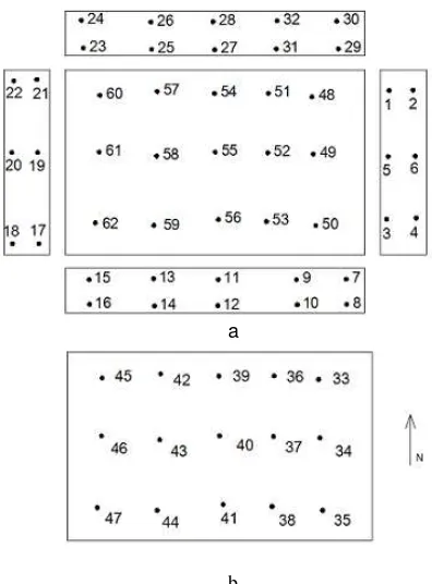
62 points (circular black-and-white targets) distributed homogeneously throughout a large calibration room (approximately 15 m x 8 m x 3 m), covering the scanner’s entire field of view, including the ceiling (up to the zenith) and the floor (up to the minimum elevation angle below the horizon plane) define the object space reference network (Fig. 1). The network design has to be strong enough to remove correlations between the additional parameters. The measurement of the target points was done with a Leica Total Station TS-30 with nominal accuracies of 0.5” for the angular measurements and 0.5 mm for the ranges.
a
b
Figure 1. Reference network: a) view of the floor and the walls projected on each side; b) view of the ceiling.
A single equilateral triangulation was surveyed to set the targeted reference network. Front and back angular observations to each target were made from the three different stations, and the distances between the stations were accurately measured (up
to eight times) to fix the network scale. First, a free network adjustment was developed to determine the best datum (the frame materialized by the triangle). Once settled the main triangle, the resolution of the rest of the reference network was constrained to this datum by a least squares adjustment. The accuracy achieved in the co-ordinates of the targeted points was ≤ 1 mm in all three axes.
4.2 Information about the two laser scanner systems The calibration performance was carried out with two midrange time-of-flight laser scanners (Fig. 2): a pulse-based Leica HDS3000 (formerly Cyrax 3000); and an amplitude-modulated continuous wave FARO LS 880. The former is a hybrid laser scanner, with a FoV of 360º in the horizontal plane, and 135º from the zenith in the vertical direction. The latter corresponds to a panoramic architecture. It means that the horizontal rotation interval is limited to the interval 0-180º, while the vertical angle ranges from the minimum angle in the front side (70º below the horizontal plane) to the same elevation angle at the back, passing through the zenith, i.e. a total of 320º. The FoV is an important factor to consider because the parameterization of observed equations has to agree with the true observation angles measured by the laser scanner. The technical data supplied by the manufacturer for the Leica HDS3000 specifies an accuracy of 4 mm for the range measurement and 60 µrad for the angles. For the FARO 880, the co-ordinate position accuracy is estimated as 3 mm at 25 m.
The scanner architecture effects the correlation between additional parameters, especially for the horizontal angle observations. In addition, the FARO and Leica scanner collect data at significantly different rates, and therefore the target observations were collected differently for each. For the FARO 880, large-resolution full domes were captured inside the calibration room due to its fast data acquisition. Scanning full domes with the older Leica HDS 3000 would be extremely slow. Thus the black-and-white targets were measured one-by-one and their centroids determined within Leica Cyclone-by-one software in order to accelerate the measurements and achieve greater precision when computing the reference network.
4.3 Laser scanning data acquisition strategy for calibration Development of a specific data acquisition strategy is a necessity to maximize the observability and recovery of the additional parameters. In Bae and Lichti (2007) a simulation is proposed in order to find the optimal scan positions. Herein, a minimum of four scanner stations are proposed, with the zero line of the instrument aligned in orthogonal directions among stations (Fig. 2); each scanner station height should also vary, and a mildly tilted scan improves precision of the collimation axis error over a network comprising all nominally-level scans for terrestrial laser scanners (Lichti et al., 2011; Chow et al., 2013).
The data acquisition strategy has two goals: first, to provide enough redundancy for the adjustment; second, to mitigate the presence of implicit linear correlations between some orientation parameters that otherwise could interfere in the convergence of the adjustment. The influence of the number of scans on the correlations is also checked in Reshetyuk (2009; 2010). The network design is also important, introducing correlations into the adjustment in cases of weak geometry. The size of the calibration room is also relevant, playing a key role to determine the range offset (a0), in fact a wide range of observed distances is required (Lichti, 2010).
a
b
Figure 2. Laser scanner stations and orientations of the zero lines inside the calibration room: a) Leica HDS3000; b) FARO
LS 880.
Correlations are especially prevalent among internal orientation (additional) parameters themselves, as well as with some EOP. Correlation between rangefinder offset and its scale factor can reach a correlation coefficient of 0.95 in some cases; horizontal angle parameters can be also problematic with coefficients greater than 0.5, and the vertical circle index error is perfectly correlated (c = -1) with elevation angle scale in hybrid models. Main problems in correlation between additional parameters and external orientation happen between horizontal angle (collimation axis error and horizontal angle scale) and kappa angle (rotation over Z axis) especially in hybrid devices, and vertical circle index error with Z translation (c ≈ 0.8) and to a lesser extent (c ≈ 0.5) with omega and phi angles (rotations on X and Y axes respectively). Some of these correlations may be unavoidable. In fact, the reference frame set by both target distribution and number of scan stations, as well as FoV of the instrument and dual axis compensator also can introduce additional parameter correlations. Lichti (2009; 2010) and Lichti et al. (2011) analyse the influence of the instrument’s architecture (FoV) on the correlations. Reducing the correlation to some of the additional parameters requires introducing constraints on both the parameters and the EOPs (Lichti, 2007; Reshetyuk, 2009), or a more favourable approach considering a reduced collimation axis error model in hybrid-style terrestrial laser scanners (Lichti et al., 2011).
5. ANALYSIS OF RESULTS 5.1 Leica HDS 3000
The geometric calibration approach started with a point cloud registration of the four scan stations, achieving RMS of the residuals on the control points equal to 0.002 m. Next, outlier observations were eliminated, and statistical testing was performed to select the significant additional parameters using the strategy presented in Section 4. Once the outliers are detected and removed, an initial adjustment is carried out with the complete set of parameters. Later, a progressive elimination
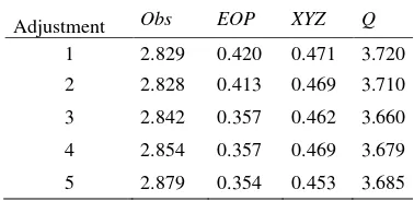
of additional parameters is performed. Specifically, the non-significant parameters are removed, starting with the lower significant probabilities, 70%, up to 99.9%. The results are presented in Table 1.
Adjustment 1 corresponds with the complete parameterization. After removing parameters with low statistical relevance (up to 70%), the estimators exhibit a slight improvement that is increased with the acceptance of additional parameters over 80% (Adjustment 3, Table 1). Finally, only those additional parameters with a confidence level of 99.9% will remain. As confirmed by the quality estimators, the best results in both the external orientation and the reference points are achieved in Adjustment 5, at the cost of a small loss in the accuracy of the observables. The estimated accuracies achieved in the absence of additional parameters (without APs), with all APs (Adjustment 1) and with the significant parameters over 99.9% (Adjustment 5) are presented in table 2. It is worth noting the significant improvement in the range accuracy owing to the offset error correction (over 1.5 mm) and the scale factor.
Table 1.Geometric calibration quality estimators obtained for the Leica HDS 3000 with distinct parameterization: 1) All APs;
2) Significant APs, p > 70%; 3) Significant APs, p >80%; 4) Significant APs, p >90%; 5) Significant APs, p >99.9%.
Adjustment Obs EOP XYZ Q 1 2.829 0.420 0.471 3.720
2 2.828 0.413 0.469 3.710
3 2.842 0.357 0.462 3.660
4 2.854 0.357 0.469 3.679
5 2.879 0.354 0.453 3.685
Table 2. A posteriori accuracies achieved for the observables based on two parameterizations. Improvement ratios between
first and second columns (Adjustment 1).
Without APs
All APs
APs p > 99%
Improvement (%)
ρ (mm) 3.10 0.96 0.97 69.0
Ѳ (“) 8.52 8.18 8.30 3.9
α (“) 21.61 20.03 20.15 7.3
Once the final set of additional parameters is considered (Adjustment 5), observables are corrected and point cloud registration is re-calculated. RMS values and improvements are presented in Table 3 considering both the original observables and the corrected observables after Adjustment 5.
In order to assess the improvement in object space, a set of ten check points was used in the adjustment with the purpose of checking the validity of the resulting calibration. These ten check points were selected randomly within the network, in order to keep control on every wall of the calibration room. The check point results are shown in Table 4 (percentage magnitudes).
Table 3. RMS of residuals on the targets obtained in the registration of each scan station before calibration (Initial RMS making use of the original scanned point cloud for the external
orientation, column 2) and RMS after calibration (after correcting the measurements with APs and re-calculating the
external orientation, Adjustment 5, column 3).
LEICA HDS 3000
Scan Initial RMS (m)
Posteriori RMS (m)
Improvement (%)
1 0.0032 0.0008 74.50%
2 0.0035 0.0009 74.18%
3 0.0035 0.0009 73.53%
4 0.0031 0.0008 75.24%
Table 4. Percentage of improvement associated to each check point in its respective scan for the Leica HDS 3000.
Point Id.
Scan 1 (%)
Scan 2 (%)
Scan 3 (%)
Scan 4 (%)
Average (%)
2 58.49 31.25 77.08 72.34 59.79
5 87.50 60.71 80.00 86.49 78.68
7 -11.11 75.76 22.73 47.06 33.61
12 52.63 50.00 33.33 68.42 51.10
17 75.00 67.69 85.11 86.96 78.69
22 90.00 77.14 68.63 81.82 79.40
25 75.86 78.13 88.57 62.50 76.26
30 40.91 57.69 71.15 87.80 64.39
58 -40.00 81.48 89.66 - 43.71
46 30.77 - 23.53 - 27.15
The improvement ratio ranges from 27.15% up to 79.40%. The averages are fairly homogeneous, although points 7 and 58 in Scan 1 do show a decrease in accuracy. It should be noted that this ratio is highly conditioned by the quality of the check point and may be adversely affected by undetected outliers. In any case, the improvement achieved in the process is closely reflected with a median value of 59.3% which confirms the improvement gained with the geometric calibration.
5.2 FARO 880
The geometric calibration is executed for the FARO in a similar manner as presented for the Leica. After registration (RMS errors of: 0.0018, 0.0022, 0.0025 and 0.0025 m for the four scans, respectively), the elimination of outliers took place without calibration parameters, and afterwards with the whole set of additional parameters. Once the observables were filtered, the search for significant parameters began again. The change in the quality index with different additional parameters is shown in Table 5.
Table 5. Geometric calibration quality estimators obtained for the FARO LS 880 with distinct parameterization: 1) All APs; 2)
Significant APs, p > 70%; 3) Significant APs, p >80%; 4) Significant APs, p >95%; 5) Significant APs, p >99%; 6)
Significant APs, p >99.9%.
Adjustment Obs EOP XYZ Q
1 (All APs) 2.965 2.636 1.543 7.144
2 (APs > 70%) 2.966 2.549 1.530 7.045
3 (APs > 80%) 3.001 2.506 2.094 7.601
4 (APs > 95%) 3.115 1.939 2.150 7.205
5 (APs > 99%) 3.130 1.935 1.564 6.629
6 (APs > 99.9%) 3.340 2.048 2.298 7.686
From the complete parameterization, the calibration parameters of minor statistical importance were iteratively suppressed from the model, until the best estimation was achieved. The evolution of the geometric calibration is shown in Table 5. The first adjustment corresponds with the full calibration (21 APs). From this, those coefficients whose t-test value indicates low significance were deleted, resulting in Adjustment number 2. Subsequently, the significant threshold increased up to Adjustment 6 (p > 99.9%). As it can be confirmed with the two sets of best probability, significant differences exist in accuracy terms. Thus, according to the computed quality estimators, parameterization number 6 shows a certain loss in the three fields of interest. Therefore Adjustment 5 is proposed as the best geometric parameterization with 9 APs. Table 6 shows the error magnitudes and the improvement ratios achieved after the geometric calibration. Table 7 shows the improvements in the accuracy of the observations before and after self-calibration with p>99% (Adjustment 5).
Table 6. RMS of residuals on the targets calculated for each scan station before calibration (Initial RMS after registration, column 2) and RMS after calibration (Adjustment 5, column 3).
FARO 880
Scan
Initial RMS (m)
Posteriori RMS (m)
Improvement (%)
1 0.0022 0.0014 34.76%
2 0.0027 0.0018 33.41%
3 0.0028 0.0018 34.45%
4 0.0029 0.0018 38.09%
Table 7. A priori versus a posteriori accuracies achieved on the observables (without APs vs Adjustment 5).
Without APs
All APs
APs p > 99%
Improvement (%)
ρ (mm) 1.66 1.18 1.18 28.9
Ѳ (“) 86.27 69.94 72.73 15.7
α (“) 61.54 51.65 52.20 15.2
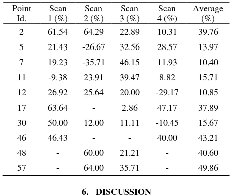
Testing and evaluation of the improvement achieved on the check points can be seen in Table 8. It ranges from 10.40 % up to 49.86 %, with a median value of 27.79%.
Table 8: Percentage of improvement associated to each check point in its respective scan for the FARO LS 880.
Point
Based on the magnitudes of the improvements achieved on both terrestrial laser scanners, it is possible to confirm the benefits of geometric calibration to yield estimates below 1 mm on ideal conditions (i.e. calibration room full of targets and short ranges). The results for the FARO instrument are not as good as shown in Lichti and Licht (2006), where the achieved ratios are significantly better (36% for the range, 30% for the horizontal direction, and 31% for the elevation angle). In Lichti et al. (2007) a comparison of the residuals resulting of the adjustment with and without parameters is raised to quantify the improvement of the self-calibrations, showing an increase in accuracy only in the horizontal angle (a 14% in the horizontal direction versus 1% in the range and the elevation angle). In the case of the experiment performed in González-Aguilera et al. (2011) for two different pulse-based scanners (Riegl LMS-Z390i and Trimble GX200) the improvements reached only were significant for the Trimble instrument (33% for the range, 53 % for the horizontal angles and 67% for the elevation).
Considering the achieved improvement ratios, mainly in the Leica HDS 3000, it seems clear that the process for detecting and removing systematic errors in laser scanner measurements is mandatory for the success of the project. The existence of multiple systematic errors in the original point clouds is highlighted in this paper. Solving for a significant set of additional parameters should not be neglected before handling both point clouds and meshes.
To get error-free systematic errors from the calibrated terrestrial laser scanner, raw Cartesian co-ordinates delivered by the TLS have to be transformed into polar coordinates (unless the instrument delivers them) to correct the raw measurements. Afterwards, updated Cartesian co-ordinates will be computed. This operation will yield better output and improve other activities such as filtering and segmentation. The importance of the geometric calibration process will be particularly evident in those cases where several point clouds need to be merged/registered. As normally most laser scanning projects require more than two scan stations. Geometric calibration will be crucial at the registration step when merging all the point clouds onto a single reference system. This step is required to reduce the point cloud noise without smoothing. And this issue is independent of the survey. Nevertheless, the geometric calibration step is mandatory for quality control and monitoring
of continuous planar features such as walls, ceilings and floors. This process may also allow the user to maximize the accuracy of older, worn laser scanning equipment. For example, the old Leica HDS 3000 calibrated herein improved its precision up to 70%. The significant positive (and sometimes negative) improvements in Table 8 are probably due to the own instabilities between scans of the FARO PHOTON, despite in general the improvement goes up from a minimum of 10.24% on point 7 up to 49.86% on point 57. García-San-Miguel and Lerma (2013) report on this problem as well as the unexpected lack of Gaussian distribution of errors on the new versions of the FARO laser scanner, the FARO FOCUS 3D.
About the statistical process developed in this paper, there are a few important facts that ensure the quality of the parameterization. Removing the correlations between parameters is confirmed in different papers (Licthi, 2010; Reshetyuk, 2009; 2010), but the other statistical strategies presented herein are also relevant to succeed in the best parameterization. The incorporation of the analysis of the variances and the study of the internal reliability is considered crucial to attain the best calibration. In fact, appropriate weighting is not only required for the whole adjustment but for each equation. The strict compliance with the global test of the model is imperative to ensure the validity of the parameterization; improper weighting can lead to erroneous results. Furthermore, the quality estimators proposed herein helped the other statistical tools to define the significant parameters in some particular cases. For example, it is demonstrated that for the FARO LS 880 the 99% probability parameterization yielded better estimates than the 99.9% one. Thus, a reliable parameterization requires all the tools presented herein; none of them can be excluded to provide a confidence solution.
7. CONCLUSIONS
This paper presents a geometric calibration strategy used to improve the performance of hybrid and panoramic terrestrial laser scanners based on statistical analysis through a dimensionless quality index. The presented approach makes use of a reference network of point targets. Geometric self-calibration can be undertaken to deliver error-free systematic measurements. It requires a deep mathematical and statistical knowledge and a balance between trying to minimize correlations between parameters and maximize reliability based on statistical quality estimators. A comprehensive self-calibration strategy is mandatory to achieve the best parameterization.
The parameterization describing the systematic errors in range, horizontal and elevation angles is scanner-based, and depends not only in the architecture. The results of calibrating two time-of-flight laser scanners are presented, one pulse-based Leica HDS 3000 and a continuous wave FARO LS 880. The improvement in the accuracy of the check points of the former was in average almost 60% (59.3%), while the latter averaged 27%. Higher improvements ratios were achieved both on the RMS registration errors and on the observables with an appropriate set of additional parameters. The dimensionless quality index estimators presented herein to determine the best set of additional parameters are highly recommended for the successful calibration of terrestrial laser scanners: not only improvements in observables should be considered but also improvements in exterior orientation parameters and ground control points. Geometric calibration of terrestrial laser scanners ISPRS Annals of the Photogrammetry, Remote Sensing and Spatial Information Sciences, Volume II-5, 2014
should not be neglected to improve output data sets, simplifying subsequent data processing such as filtering and smoothing.
The stability of the additional parameters over time and under different scenarios, indoor versus outdoor, short versus long range will be further estimated in the future. Nevertheless, larger than usual indirect registration errors are simple evidences that should alarm users about the deterioration performance of the laser scanning system. Therefore, a geometric self-calibration strategy should not be underestimated.
REFERENCES
Amiri Parian, J., Gruen A., 2005. Integrated laser scanner and intensity image calibration and accuracy assessment. The International Archives of Photogrammetry, Remote Sensing and Spatial Information Sciences, Vol. 36, Part 3/W52, pp. 14-19.
Amiri Parian, J., Gruen, A., 2010. Sensor modeling, self-calibration and accuracy testing of panoramic cameras and laser scanners. ISPRS Journal of Photogrammetry and Remote Sensing, 65 (1), 60-76.
Baarda, W., 1968. A testing procedure for use in geodetic networks. Publications on Geodesy 9, 2(5), Delft, Netherlands, 97 p.
Bae, K.-H., Lichti, D.D., 2007. On-site self-calibration using planar features for terrestrial laser scanners. The International Archives of Photogrammetry, Remote Sensing and Spatial Information Sciences, Vol. 36, Part 3/W52, pp. 14-19.
Baselga, S., 2011. Nonexistence of Rigorous Test for Multiple Outlier detection in Least-Squares Adjustment. Journal of Surveying Engineering, 137(3):109-112.
Chow, J.C.K., Lichti, D.D., Glennie, C., 2011. Point-based versus plane-based self-calibration of static terrestrial laser scanners. International Archives of the Photogrammetry, Remote Sensing and Spatial Information Sciences, Vol. 38, Part 5/W12, pp. 121-126.
Chow, J.C.K., Lichti, D.D., Glennie, C., Hartzell, P., 2013. Improvements to and Comparison of Static Terrestrial LiDAR Self-Calibration Methods. Sensors, 2013, 13(6), 7224-7249
García-San-Miguel, D., Lerma, J.L., 2013. Geometric calibration of a terrestrial laser scanner with local additional parameters: An automatic strategy. ISPRS Journal of Photogrammetry and Remote Sensing, 79:122-136.
Gielsdorf, F., Rietdorf, A., Gruendig, L., 2004. A concept for the calibration of terrestrial laser scanners. In: Proceedings FIG Working Week, Athens, Greece, 22-27.
Glennie, C., 2012. Calibration and kinematic Analysis of the Velodyne HDL-64E S2 Lidar Sensor. Photogrammetric Engineering & Remote Sensing, 78(4):339-347.
Glennie, C., Lichti, D.D.,, 2010. Static Calibration and Analysis of the Velodyne HDL-64E S2 for High Accuracy Mobile Scanning. Remote Sensing, 2(6):1610-1624.
González-Aguilera, D., Rodriguez-Gonzálvez, P., Armesto, J., Arias, P., 2011. Trimble GX200 and Riegle LMS-Z390i. Optic Express, 19(3):2676-2693.
Hofmann-Wellenhof, B., Lichtenegger, H, Collins, J., 2001. Global Positioning System: Theory and Practice (5th rev. ed.), Springer-Verlag, Wien, 382 p.
Kersten, T.P., Sternberg H., Mechelke, K., 2005. Investigations into the accuracy behaviour of the terrestrial laser scanning system Mensi GS10. Optical 3-D Measurement Techniques VII, Vol. I, pp. 122-131.
Kraus, K., Jansa, J., Krager, H., 1997. Photogrammetry Volume 2, Advanced Methods and Applications (4th ed.), Dümmler, Bonn, Germany, 466 p.
Lichti, D.D., 2000. Calibrating and testing of a terrestrial laser scanner. International Archives of Photogrammetry, Remote Sensing and Spatial Information Sciences, Vol. 33, pp. 485-492.
Lichti, D.D., 2007. Error modeling, calibration and analysis of an AM-CW terrestrial laser scanner system. ISPRS Journal of Photogrammetry and Remote Sensing, 61(5):307-324.
Lichti, D.D., 2009. The impact of angle parameterization on terrestrial laser scanner self-calibration. International Archives of the Photogrammetry, Remote Sensing and Spatial Information Science, Vol. 38, Part 3/W8, pp. 171-176.
Lichti, D.D., 2010. Terrestrial laser scanner self-calibration: correlation sources and their mitigation. ISPRS Journal of Photogrammetry and Remote Sensing, 65:93-102.
Lichti, D.D., Chow, J., Lahamy, H., 2011. Parameter de-correlation and model-identification in hybrid-style terrestrial laser scanner self-calibration. ISPRS Journal of Photogrammetry and Remote Sensing, 66 (3), 317-326.
Lichti, D.D., Licht, M.G., 2006. Experiences with terrestrial laser scanner modeling and accuracy assessment. The International Archives of Photogrammetry, Remote Sensing and Spatial Information Sciences, Vol. 36, Part 5, pp. 155–160.
Lichti, D.D., Brüstle S., Franke, J., 2007. Self-calibration and analysis of the surphaser 25HS 3D scanner. In: Proceedings of FIG Working Week, Hong Kong SAR, China, 13-17, 13 p.
Pope, A.J., 1976. The statistics of residuals and the detection of outliers. NOAA Technical Report NOS 65 NGS 1, National Ocean Service, National Geodetic Survey, Rockville, MD, 133 p.
Reshetyuk, Y., 2009. Self-calibration and direct georeferencing in terrestrial laser scanning. Ph.D. dissertation, Royal Institute of Technology (KTH), Stockholm, Sweden, 162 p.
Reshetyuk, Y., 2010. A unified approach to self-calibration of terrestrial laser scanners. ISPRS Journal of Photogrammetry and Remote Sensing, 65(5):445-456.
Schneider, D., 2009. Calibration of a Riegl LMS-Z429i based on a multi-station adjustment and a geometric model with additional parameters. International Archives of Photogrammetry, Remote Sensing and Spatial Information Sciences, Vol. 38, Part 3/W8, pp.177-182.
Soudarissanane, S., Lindenbergh, R., Menenti, M., Teunissen, P., 2011. Scanning geometry: Influencing factor on the quality of terrestrial laser scanning points. ISPRS Journal of Photogrammetry and Remote Sensing, 66(4) 389-399.