A COMPARISON OF LIDAR REFLECTANCE AND RADIOMETRICALLY CALIBRATED
HYPERSPECTRAL IMAGERY
A. Roncata,∗, C. Briesea,b, N. Pfeifera
aResearch Groups Photogrammetry and Remote Sensing, Department of Geodesy and Geoinformation, TU Wien, Vienna, Austria ✭❛♥❞r❡❛s✳r♦♥❝❛t✱❝❤r✐st✐❛♥✳❜r✐❡s❡✱♥♦r❜❡rt✳♣❢❡✐❢❡r✮❅❣❡♦✳t✉✇✐❡♥✳❛❝✳❛t,✇✇✇✳❣❡♦✳t✉✇✐❡♥✳❛❝✳❛t
b
EODC Earth Observation Data Centre for Water Resources Monitoring GmbH, Vienna, Austria ❝❤r✐st✐❛♥✳❜r✐❡s❡❅❡♦❞❝✳❡✉,✇✇✇✳❡♦❞❝✳❡✉
Commission VII, WG VII/6
KEY WORDS:Radiometry, Calibration, Laser Scanning, Hyperspectral
ABSTRACT:
In order to retrieve results comparable under different flight parameters and among different flight campaigns, passive remote sensing data such as hyperspectral imagery need to undergo a radiometric calibration. While this calibration, aiming at the derivation of phys-ically meaningful surface attributes such as a reflectance value, is quite cumbersome for passively sensed data and relies on a number of external parameters, the situation is by far less complicated for active remote sensing techniques such as lidar.
This fact motivates the investigation of the suitability of full-waveform lidar as a “single-wavelength reflectometer” to support radiomet-ric calibration of hyperspectral imagery. In this paper, this suitability was investigated by means of an airborne hyperspectral imagery campaign and an airborne lidar campaign recorded over the same area. Criteria are given to assess diffuse reflectance behaviour; the distribution of reflectance derived by the two techniques were found comparable in four test areas where these criteria were met. This is a promising result especially in the context of current developments of multi-spectral lidar systems.
1. INTRODUCTION
Commercial full-waveform lidar systems have become ever in-creasingly available and used for the production of high-resolu-tion 3D topographic informahigh-resolu-tion in the past decade. Full-wave-form lidar additionally inherits the possibility of assigning phys-ically meaningful target attributes, e.g. the backscatter cross-sec-tion or a diffuse-reflectance value, to the resulting 3D point cloud in the same spatial resolution. This allows for the derivation of quantities comparable for different sensors, emitted laser ener-gies, other flight-campaign parameters and acquisition dates.
While the process of radiometric calibration for lidar data as an active remote sensing technique is rather straightforward (Wag-ner, 2010, Briese et al., 2012), for passively sensed optical data such as hyperspectral imagery (HSI), several additional variables have to be considered. Concerning the airborne case, these vari-ables are typically given in resolutions much coarser than the ground sampling distance of the optical sensor.
Airborne lidar, also known as airborne laser scanning (ALS), has already proven to be a valuable geometric source for facilitat-ing radiometric calibration of hyperspectral imagery (Schneider et al., 2014). Beyond that, the aforementioned lidar-derived sur-face attributes, especially diffuse reflectance, may also serve as a radiometric input for calibrating hyperspectral data in an ac-cording wavelength domain, acting as a “single-wavelength re-flectometer” in an area-wide sense. In this study, we present a method for validating the lidar-derived diffuse surface reflectance and and its comparison to according values calculated from HSI data. The hypothesis is evaluated by means of an extended full-waveform lidar campaign and an HSI campaign, both recorded over the Lägern area, located northwest of Zurich, Switzerland.
The paper is organized as follows: The underlying physical and mathematical frameworks for radiometric calibration of both
li-∗Corresponding author.
dar and passively sensed data are presented in Section 2, followed by the method for comparing the reflectances retrieved by each of this techniques in Section 3. The subsequent section describes the used data sets. Results are given in Section 5; conclusions are drawn in the last section.
2. THEORY
In this section, we will present the physical-mathematical frame-work for radiometric calibration for both lidar and passively sen-sed optical data.
2.1 Radiometric Calibration of Lidar Data
The basic relation of the transmitted power of a laser pulsePt(t)
and the recorded echo powerPe(t)is given by the radar equation
(Jelalian, 1992, Wagner, 2010):
Pe(t) =
D2
r 4πR4β2
t
Pt
t−2R
vg
σ ηSYSηATM, (1)
withβtbeing the beamwidth of the transmitted signal,R
denot-ing the distance from the sensor to the target,tthe travel time,
vg the group velocity of the laser ray (approx. speed of light
in vacuum), Dr the receiving aperture diameter,ηSYS the sys-tem transmission factor andηATMthe atmospheric transmission factor. Thescattering cross-sectionσ(inm2
) summarizes target characteristics:
σ:= 4π ΩS
ρALcosϑ. (2)
The termAL[m2]is the area of the laser footprint, i.e. the area
formed by the intersection of the cone and a sphere with centre at the laser’s position and radiusRcorresponding to the distance from the laser to the target, whileΩS[sr]is the solid angle of the
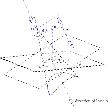
angle, i.e. the angle formed by the direction of the laser beam and the local surface normal of the target surface; see Figure 1.
O nε R
Figure 1: Geometric parameters of the radar equation. The angle
ϑformed by the laser ray and the normal of of the target planeε
is called incidence angle (Roncat et al., 2012).
In a monostatic configuration, i.e. the transmitter and receiver be-ing close together, σis to be considered asbackscatter cross-section. This is the case for practically all airborne lidar systems. If the target surface exhibits a diffuse reflectance behaviour, the scattering solid angleΩS=πand the diffuse surface reflectance
ρdis derived as
ρd=
σ
4ALcosϑ
.
The retrieval ofσand/orρdis known as radiometric calibration.
For this purpose, unknown but constant quantities are summa-rized ascalibration constant, determined by means of reference targets which might be surfaces of (assumed) known and con-stant reflectance (Wagner et al., 2006), natural or artificial sur-faces with calibrated reflectance behaviour (Lehner and Briese, 2010, Kaasalainen et al., 2009).
If the last factor in Equation (1),ηATM, can be assumed as con-stant throughout the flight campaign, it is included in the calibra-tion constant and not determined independently. If such an as-sumption does not hold,ηATMcan be formulated as a function of the rangeRand of an (constant) atmospheric attenuation coeffi-cienta[dB/km](Höfle and Pfeifer, 2007):
ηATM(R) = 10 −
2Ra
10000,
or, in the case of a more complex atmospheric situation, be cal-culated per target w.r.t. to atmospheric parameters, flight altitude and terrain elevation by applying look-up tables as e.g. imple-mented in the ATCOR software (Richter and Schläpfer, 2016). An assessment of the variation ofηATMfor the dataset investi-gated in this study is given in Section 4.
The actual formulation of the calibration constant and sequence of calibration steps may vary w.r.t. (a) which input data is avail-able, e.g. an intensity value per point, amplitude and echo width derived by full-waveform data, additional amplitude and width of the transmitted signal, or a deconvolved echo waveform. Further: (b) which quantities can be assumed as constants and (c) which
quantity is sought as result of radiometric calibration (Briese et al., 2012, Roncat, 2014). Additionally toσandρd, also a
normal-ized backscatter cross-sectionσ0
and a backscatter coefficientγ
(both unitless) may be the quantity of interest in radiometric cal-ibration.
While the backscatter cross-sectionσcan be derived from data only related to the single 3D point of interest itself, the diffuse reflectance requires knowledge of the spatial neighbourhood of this point, expressed e.g. by the local surface-normal vector, com-monly derived using the 3D point cloud of the same lidar cam-paign.
2.2 Radiometric Calibration of passively sensed optical Data
In addition to the aforementioned factors to be considered in ra-diometric calibration, passively sensed data are also dependent on various other quantities. In a first step, a gain factor and an offset have to be applied, transferring the digitized pixel values to at-sensor radiancesLλ, given inW/(m
2
srµm)or equivalent. To derive further the surface reflectanceρ, the following parameters are to be considered (Moran et al., 1992, Chander et al., 2009):
• the mean solar exo-atmospheric irradiance,
• the solar zenith angle,
• the Earth-Sun distance,
• the path radiance,
• the atmospheric transmittance in viewing and illumination direction, resp., and
• the downwelling diffuse irradiance.
Their values are commonly given in models of coarser resolution than the one of imagery data.
3. METHOD
In order to support HSI radiometric calibration by lidar-derived reflectance, areas are to be determined where a diffuse surface reflectance can be assumed, i.e. where the reflectance is indepen-dent of the viewing direction of the sensor. This is an important prerequisite as the surfaces are likely to be viewed from different positions in a lidar and an HSI campaign, resp.
As a first criterion, the lidar-derived reflectance is only valid for extended targets, i.e. the target area exceeding the the one of the laser beam footprint. Therefore, only single echoes per laser shot can be taken into consideration. Additionally, the echo ratio is to be considered. This quantity is the number of points in the 3D neighbourhood (i.e. a sphere) of a (grid) point,n3D, divided by the number of pointsn2Din the 2D neighbourhood of this point, i.e. a cylinder of the same radius (Höfle et al., 2009):
ER [%] =n3D
n2D
·100, (3)
withn3D≤n2D. The echo ratio can be considered as an opacity measure in vertical direction. See Figure 2 for explanatory exam-ples.
Figure 2: Definition of the Echo RatioER(Höfle et al., 2009).
compare one flight strip to the other. In case a certain threshold of the absolute value of their difference is exceeded, the hypothe-sis of diffuse reflectance is to be rejected. Moreover, the assump-tion of a well-defined normal vector of the target surface can be evaluated using the standard error of unit weightσ0of the nor-mal vector calculation. Thisσ0 can be considered as a measure of surface roughness. Only where all three criteria are met:
(a) extended and opaque targets,
(b) isotropic reflectance behaviour, and
(c) a well-defined surface-normal vector,
the reflectance behaviour of the surface may be considered as dif-fuse.
4. DATA SETS
The data investigated in this study were recorded over the Lägern area, a wooded mountainous area in the Jura mountains, located northwest of Zurich, Switzerland. The lidar campaign was carried out on August 1, 2010 using a RIEGL LMS-Q680 full-waveform instrument, operating at a wavelength of1,550 nm(Riegl LMS, 2016). The point density was approx. 50 points perm2
; The cam-paign consisted of 15 flight strips and covered an area of about
12.5 km2 .
Hyperspectral imagery data were recorded over the Lägern area on July 18, 2014 using an APEX sensor (Hueni et al., 2009); the wavelengths ranged from400 nm−2,500 nm. The wavelength of the band used for comparison to the lidar data was1,551 nm
(FWHM = 22 nm). The spatial resolution of the HSI data was about1.5 mat ground; reflectance values were resampled to a
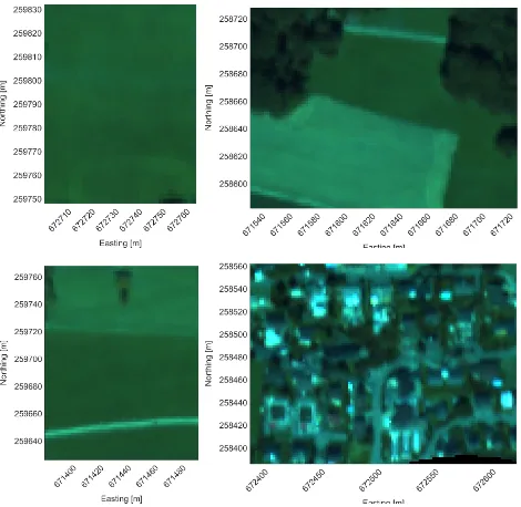
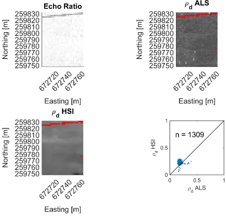
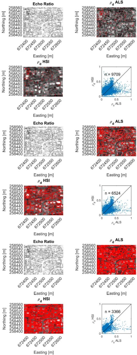
2 mgrid in the Swiss National Coordinate System CH1903. The overlapping area of the two campaigns is mostly forested but con-tains grasslands, fields and built-up areas as well. Based on the criteria for assessing diffuse surface reflectance in lidar data pre-sented in the previous section, four test areas were chosen, illus-trated by red rectangles in Figure 4. The respective reflectance values were resampled to a2 mgrid. A description of the test areas in detail (see also Figure 3):
Test area 1: area of homogeneous reflectance behaviour. The dis-tribution of the reflectance in both datasets, expressed by the median and theσMAD, was assumed to be uni-modal and comparable.
Test areas 2 and 3: areas covered with surface types of differ-ent reflectance, i.e. roads, grassland and fields. In addition to the distribution, the linear relationship between the two datasets, expressed by the coefficient of determinationR2
, was investigated as well.
Test area 4: a more complex scene in a built-up area where the dependence of median andσMADon a minimum echo ratio was assessed.
An overview of the whole campaigns’ setup is shown in Figure 4.
Figure 3: The four test areas in detail, shown as RGB true-color composite of the according HSI reflectances. Top left: test area 1, bottom left: test area 2. Top right: test area 3, bottom right: test area 4.
The radiometric calibration of the lidar dataset and the calculation of normal vectors on a per-point level as well as the interpolation of rasters for reflectance, echo ratio and strip differences were performed using the lidar software suite OPALS (OPALS, 2016), developed by TU Wien. The HSI reflectance grid was delivered by University of Zurich.
Concerning the variation of the atmospheric transmission coeffi-cientηATMwithin the lidar dataset, the maximum relative differ-ences to a mean value ofηATM were assessed, applying (a) an attenuation coefficient ofa= 0.22 dB/kmand (b) atmospheric look-up tables, resp. In both cases, the relative variations did not exceed±2%. Therefore,ηATMwas regarded as constant for this dataset.
5. RESULTS
The four test areas showed that the variations in the lidar-derived reflectances, expressed byσMAD, were slightly higher than the ones in the HSI-derived reflectances. This might be due to the higher spatial resolution of the original raw lidar data and the resulting capability of assessing reflectance variations in higher detail. The numerical results are given in Table 1.
Test areas 2 and 3 showed R2
values of0.53and 0.59for the lidar- and HSI-derived reflectance, resp. In both test areas, a slight increase inR2
Figure 4: Overview of the lidar and the HSI campaign recorded over the Lägern area. An RGB composite of the according HSI reflectances is shown in the background. The outlines of the lidar strips are shown in black and the four test areas are depicted by red rectangles. Coordinate system: Swiss National Grid CH1903.
lidar HSI
test area median σMAD median σMAD
1 0.184 0.017 0.221 0.020
2 0.164 0.049 0.180 0.030
3 0.219 0.133 0.215 0.110
4 0.172 0.087 0.176 0.059
Table 1: Reflectance distributions for the four test areas, evaluated for a minimum echo ratio of75% each. Detailed results w.r.t. varying minimum echo ratio for test area 4 are given in Table 2.
Figure 5: Results for test area 1, evaluated for a minimum echo ratio of75%. Reflectance values are shown in grayscale from 0 (black) to 1 (white) and the echo ratio is visualized analogously. Pixels excluded from the analysis due to an echo ratio below the threshold are shown in red.
Figure 6: Results for test area 2, evaluated for a minimum echo ratio of75%. Reflectance values are shown in grayscale from 0 (black) to 1 (white) and the echo ratio is visualized analogously. Pixels excluded from the analysis due to an echo ratio below the threshold are shown in red. See also Table 2.
lidar HSI
min.ER # pixels median σMAD median σMAD
50 % 9709 0.174 0.089 0.176 0.059
55 % 9364 0.173 0.088 0.176 0.059
60 % 8880 0.174 0.089 0.176 0.059
65 % 8212 0.173 0.088 0.176 0.059
70 % 7398 0.172 0.087 0.176 0.059
75 % 6524 0.170 0.087 0.177 0.060
80 % 5701 0.167 0.086 0.178 0.060
85 % 4910 0.161 0.083 0.179 0.061
90 % 4169 0.155 0.080 0.179 0.062
95 % 3366 0.140 0.070 0.178 0.061
100 % 2457 0.128 0.065 0.174 0.057
Figure 7: Results for test area 3, evaluated for a minimum echo ratio of75%. Reflectance values are shown in grayscale from 0 (black) to 1 (white) and the echo ratio is visualized analogously. Pixels excluded from the analysis due to an echo ratio below the threshold are shown in red.
6. DISCUSSION AND OUTLOOK
This study dealt with the radiometric comparison of full-wave-form lidar and passively sensed hyperspectral data. Lidar, as an active remote sensing technique, needs by far less assumptions for performing radiometric calibration. This has led to the moti-vation for testing lidar as a “single-wavelength reflectometer” in an area-wide sense in order to support radiometric calibration of hyperspectral imagery in an according wavelength.
Criteria for the validity of the diffuse surface reflectance, assess-able in an advanced lidar-data processing, were formulated and a comparison of reflectance data was performed in four test areas within an extended airborne HSI and lidar campaign, resp.
The distribution of the reflectance, expressed by the median and theσMADvalues, was found comparable in all four test areas, giv-ing empirical evidence for the validity of the hypothesis. While this study concentrated on a single wavelength, current develop-ments of multi-spectral lidar systems (Briese et al., 2012, Hakala et al., 2012, Wallace et al., 2014) give the motivation for further research in this field.
ACKNOWLEDGEMENTS
The research leading to these results has received funding from the European Union’s 7th Framework Programme (FP7/2014– 2018) under EUFAR2 contract no. 312609.
The Lägern ALS dataset was processed at RSL (UZH) (Schneider et al., 2014).
The Lägern APEX imaging reflectometer dataset has been ac-quired within the Swiss Earth Observatory Network (SEON) pro-ject and was processed using the APEX Processing and Archiving Facility (Hueni et al., 2009).
REFERENCES
Briese, C., Pfennigbauer, M., Lehner, H., Ullrich, A., Wagner, W. and Pfeifer, N., 2012. Radiometric calibration of multi-wavelength airborne laser scanning data. In:ISPRS Annals of
the Photogrammetry, Remote Sensing and Spatial Information Sciences 1 (Part 7), Melbourne, Australia, pp. 335–340. ISSN: 1682-1750.
Chander, G., Markham, B. L. and Helder, D. L., 2009. Summary of current radiometric calibration coefficients for landsat MSS, TM, ETM+, and EO-1 ALI sensors.Remote Sensing of Environ-ment113(5), pp. 893–903.
Hakala, T., Suomalainen, J., Kaasalainen, S. and Chen, Y., 2012. Full waveform hyperspectral lidar for terrestrial laser scanning. Optics Express20(7), pp. 7119–7127.
Höfle, B. and Pfeifer, N., 2007. Correction of laser scanning in-tensity data: Data and model-driven approaches. ISPRS Journal of Photogrammetry and Remote Sensing62(6), pp. 415–433.
Höfle, B., Mücke, W., Dutter, M., Rutzinger, M. and Dorninger, P., 2009. Detection of building regions using airborne LiDAR – A new combination of raster and point cloud based GIS methods. In:Proceedings of the Geoinformatics Forum Salzburg, Salzburg, Austria, pp. 66–75.
Hueni, A., Biesemans, J., Meuleman, K., Dell’Endice, F., Schläpfer, D., Adriaensen, S., Kempenaers, S., Odermatt, D., Kneubuehler, M., Nieke, J. and Itten, K., 2009. Structure, com-ponents and interfaces of the airborne prism experiment (APEX) processing and archiving facility. IEEE Transactions in Geo-sciences and Remote Sensing47(1), pp. 29–43.
Jelalian, A. V., 1992. Laser Radar Systems. Artech House, Boston.
Kaasalainen, S., Hyyppä, H., Kukko, A., Litkey, P., Ahokas, E., Hyyppä, J., Lehner, H., Jaakkola, A., Suomalainen, J., Akujarvi, A., Kaasalainen, M. and Pyysalo, U., 2009. Radiometric cali-bration of lidar intensity with commercially available reference targets. IEEE Transactions on Geoscience and Remote Sensing 47(2), pp. 588–598.
Lehner, H. and Briese, C., 2010. Radiometric calibration of full-waveform airborne laser scanning data based on natural sur-faces. In:ISPRS Technical Commission VII Symposium 2010: 100 Years ISPRS – Advancing Remote Sensing Science. Interna-tional Archives of the Photogrammetry, Remote Sensing and Spa-tial Information Sciences38 (Part 7B), Vienna, Austria, pp. 360– 365.
Moran, M. S., Jackson, R. D., Slater, P. N. and Teillet, P. M., 1992. Evaluation of simplified procedures for retrieval of land surface reflectance factors from satellite sensor output. Remote Sensing of Environment41(2), pp. 169–184.
OPALS, 2016. Orientation and Processing of Airborne Laser Scanning data (product homepage). Department of Geodesy and Geoinformation – Research Groups Photogrammetry and Remote Sensing.❤tt♣✿✴✴❣❡♦✳t✉✇✐❡♥✳❛❝✳❛t✴♦♣❛❧s. (16 Apr. 2016).
Richter, R. and Schläpfer, D., 2016. Atmospheric/Topographic Correction for Airborne Imagery. ReSe Applications, Wil SG, Switzerland. ATCOR-4 User Guide, Version 7.0.3, March 2016 (16 Apr. 2016).
Riegl LMS, 2016. Homepage of the company RIEGL Laser Mea-surement Systems GmbH. ❤tt♣✿✴✴✇✇✇✳r✐❡❣❧✳❝♦♠. (16 Apr. 2016).
Roncat, A., 2014. Backscatter Signal Analysis of Small-Footprint Full-Waveform Lidar Data. PhD thesis. Supervisors: Norbert Pfeifer (TU Vienna), Uwe Stilla (TU Munich).
Roncat, A., Morsdorf, F., Briese, C., Wagner, W. and Pfeifer, N., 2014. Laser Pulse Interaction with Forest Canopy: Geometric and Radiometric Issues. Managing Forest Ecosystems, Vol. 27, Springer Netherlands, Dordrecht, The Netherlands, chapter 2, pp. 19–41.
Roncat, A., Pfeifer, N. and Briese, C., 2012. A linear approach for radiometric calibration of full-waveform Lidar data. In:Proc. SPIE 8537, Image and Signal Processing for Remote Sensing XVIII.
Schneider, F. D., Leiterer, R., Morsdorf, F., Gastellu-Etchegorry, J.-P., Lauret, N., Pfeifer, N. and Schaepman, M. E., 2014. Sim-ulating imaging spectrometer data: 3D forest modeling based on LiDAR and in situ data. Remote Sensing of Environment152, pp. 235–250.
Wagner, W., 2010. Radiometric calibration of small-footprint full-waveform airborne laser scanner measurements: Basic phys-ical concepts. ISPRS Journal of Photogrammetry and Remote Sensing65(6, ISPRS Centenary Celebration Issue), pp. 505–513.
Wagner, W., Ullrich, A., Ducic, V., Melzer, T. and Studnicka, N., 2006. Gaussian decomposition and calibration of a novel small-footprint full-waveform digitising airborne laser scanner. ISPRS Journal of Photogrammetry and Remote Sensing60(2), pp. 100– 112.
![BADAN LINGKUNGAN HIDUP PROVINSI SULAWESI BARAT [Paket Penyedia].](data:image/gif;base64,R0lGODlhAQABAIAAAP///wAAACH5BAEAAAAALAAAAAABAAEAAAICRAEAOw==)