An analysis of crystal dissolution fronts
in flows through porous media part 2:
incompatible boundary conditions
C.J. van Duijn
a, P. Knabner
b& R.J. Schotting
c ,*
aCWI, P.O. Box 94079, 1090 GB Amsterdam, Netherlands b
University of Erlangen-Nu¨rnberg, Institute of Applied Mathematics, Martensstraße 3, D-91058 Erlangen, Germany c
Delft University of Technology, Faculty of Civil Engineering and Geosciences, P.O. Box 5048, 2600 GA Delft, The Netherlands
(Received 2 July 1996; revised 15 April 1997; accepted 15 September 1997)
A model for transport of solutes in a porous medium participating in a dissolution– precipitation reaction, in general not in equilibrium, is studied. Ignoring diffusion– dispersion the initial value problem for piecewise constant initial states is studied, which e.g. for ionic species include a change of the ionic composition of the solution. The mathematical solution, nearly explicitly found by the method of characteristics up to the (numerical) solution of an integral equation for the position of the dissolution front, exhibits a generalized expanding plateau-structure determined by the dissolution front and the water flow (or salinity) front.q1998 Elsevier Science Limited.
Keywords: transport, shock waves, travelling wave, crystal dissolution, porous media, mathematical analysis
AMS classification: 35R35, 76S05.
1 INTRODUCTION
In this paper we continue our study of chemistry affected transport processes in porous media presented in Knabner et al.7. The transported solutes are participants in a preci-pitation–dissolution reaction, which in general is not in equilibrium, but is kinetically controlled. In Ref. 7 we have set up a model for spatially one-dimensional flow regimes. Throughout Ref. 7and the rest of this paper we refer to the solid phase as ‘crystal’ or ‘crystalline solid’, which is due to the fact that we have a specific example in mind: the dissolution of a crystalline mineral phase, which occurs as a very thin layer on the grains of the porous medium, see e.g. Willis and Rubin15. In fact, the dissolving substance may be either crystalline or amorphous. It was assumed that water content, bulk density, pore velocity q (cm s¹1) and diffusion–dispersion coefficient D (cm2s¹1) are constant. The unknown functions are u and v (mM cm¹3), where u is the molar concentration of one
of the reacting participants in solution, v is the scaled concentration of the crystalline solid (both relative to the water volume), and a third unknown w (—), which appears to take into account the nature of the dissolution reaction. For a detailed discussion on the role of w we refer to Section 2 of Ref.7. The governing equations are
]
]t(uþv)þq ]u ]x¹D
]2u
]x2¼0 (1)
]v
]t¼k{g(u; c)¹wK} (2)
0#w#1 and w(x,t)¼1 if v(x,t).0 (3)
for¹` ,x, `, t.0. The positive constants K and k are the saturation constant and a rate parameter, respectively. There is a further function c in the nonlinear function g related to the precipitation reaction. It is a conserved quantity in the sense that it satisfies the linear diffusion–advection equation
]c ]tþq
]c ]x¹D
]2c
]x2¼0 (4)
Printed in Great Britain. All rights reserved 0309-1708/98/$ - see front matter
PII: S 0 3 0 9 - 1 7 0 8 ( 9 7 ) 0 0 0 3 8 - 9
for ¹` ,x, `, t.0. The function c is solely determined by the stoichiometry of the precipitation–dissolution reaction. If this is given by
¯
M12NnM1þmM2 (5)
with positive integers n, m where M1, M2denote the species
in solution and M¯12the solid, then
c¼mc1¹nc2 (6)
where c1, c2 (mM cm
¹2) are the molar concentrations of
M1, M2. In eqns (1)–(4), c1:¼u is kept as an unknown and c2is substituted by means of6. For a spatially independent
batch situation the function c would be constant due to eqn (4), i.e. all possible values of concentrations c1(t), c2(t) lie
in an affine subspace of the one-dimensional stoichiometric subspace of the reaction, defined by the condition c¼0. In the case of ionic species, it is also possible to consider c as the scaled total (positive) electric charge of the solution. This observation helps us in distinguishing two principal situations with respect to a specification by means of initial conditions. We will consider piecewise constant states at t¼0, i.e.
We can relate these solutions to solutions of a correspond-ing boundary value problem for x.0, t.0 by considering u*, v*, c* as initial conditions and u*, v*, c*as boundary
conditions. Thus there are two situations
cp¼c
p and therefore c(x,t)¼c¼constant (8) or
cpÞc
p (9)
In eqn (8) the boundary (/initial) conditions are compatible in the sense that they belong to the same affine stoichio-metric subspace of the reaction or for ionic species that the injected fluid has the same ionic composition as the resident fluid. This situation is the only one which leads to travelling wave solutions being the subject of7. Here we concentrate on eqn (9), i.e. on incompatible boundary (/initial) condi-tions. In this paper we show how to obtain solutions of this problem in the presence of a dissolution front, i.e. a curve in the (x,t)-plane separating the region where v ¼0 from the region where v.0. To ensure that a dissolution front
exists for all t$0, one needs
vp¼0 and v
p.0 (10)
If initially crystalline solid is everywhere present in the flow domain, i.e. v* . 0 as well, then a dissolution front
may occur after a certain finite time interval. Conditions for which this happens are discussed in Section 3.2.
A typical example for the function g is, assuming the thermodynamically ideal mass action law:
g(u; c)¼un 1 ing properties to be used later on:
g(·;c) is strictly monotone increasing for u$(c/m)þ, g(·;c) is smooth for u $ (c/m)þ (at least
Lipschitz-continuous)
We need the existence of a (unique) uS¼uS(c)$(c/m)þ such that
g(u; c)¼K (12)
i.e. uSis the solubility for given c. Due to the properties of
the function g given earlier, the following condition ful-filled by eqn (11) is sufficient for eqn (12):
g c
When we require eqn (10), we additionally assume the initial states to be in chemical equilibrium, i.e.
c If solid is present everywhere, this would not lead to the appearance of a dissolution front, see eqns (63) and (64). Thus we allow in this case for an initial state for x,0 not in equilibrium, which might be thought of as the conse-quence of an instantaneous removal of saturated fluid. If dispersive transport is negligible compared to advective transport, it is reasonable to let D → 0, i.e. to cancel the corresponding terms in eqns (1)–(4) and to obtain
]
]t(uþv)þq ]u
]x¼0 (15)
for ¹` ,x, `, t .0. The initial value problem eqns
(2)–(4), (7) and (15) is known as a Riemann problem. In this paper we consider the analytical and numerical construction of a solution of this Riemann problem. For dominating advective transport, i.e. the limit D → 0 in eqn (1), we expect a good approximation of the solutions of eqns (1)–(4) and (7) ignoring only certain smoothing effects (see the comparison in Section 5). On the other hand, the treatment of the hyperbolic system by means of the method of characteristics allows a nearly explicit construction of the solution and thus gives detailed informa-tion about the qualitative structure of the soluinforma-tion. The func-tion c is found directly, without a priori knowledge about u, v and w. It follows from eqns (4) and (7) that for all t. 0
To be specific, we assume in the following
cp.c
p (17)
the monotone dependence of the solubility uS(c) on c, i.e. in
particular
uS(cp).uS(cp) (18)
In the, analysis we will not make use of this property, but in the figures it is assumed to hold true or implied by the choice of eqn (11). The outline of the paper is as follows. We first construct a solution of the Riemann problem in the case of equilibrium reactions. That is, we take ‘k ¼`’ in
eqn (2) and replace it by
g(u; c)¼wK (19)
In Section 3.1, we use the method of characteristics, to obtain an explicit representation of the solution, which still is dependent on the dissolution front x ¼ s(t). For
this free boundary, which necessarily exhibits a waiting time, we derive an integral equation, which in Section 4 is transformed to a linear Volterra equation of the second kind. This settles the existence of a solution of the integral equation, which then can be used to define a solution of the Riemann problem. In Section 3.2, this procedure is extended to the treatment of v*,v* . 0, u* # uS(c*). In
Section 5, an algorithm for the precise approximation of solutions is presented based on the above procedure.
The analysis of multi-component reactive systems with pure advective transport by means of the corresponding hyperbolic systerm has a certain tradition in the chemical engineering literature. Although the situation considered usually allows for more species and reactions then consid-ered here, most of these papers are restricted to the case of equilibrium reactions and a constant number of phases (see e.g. Walsh et al.14, Dria et al.3, Novak et al.9, Bryant et al.2, Novak et al.10, HelfErich and Klein6, Schweich et al.11(and the literature cited therein). If the non-equilibrium case is considered most authors (see e.g. Sevougian et al. 12,13) resort to numerical methods, allowing more complex and realistic situations. The main features of the simple situation studied semi-analytically in this paper are the assumption of non-equilibrium and the appeaxance of a dissolution front.
2 EQUILIBRIUM
When studying the transport process at equilibrium we replace the first order eqn (2) by the equilibrium relation (eqn (19)). Thus the equations to be analyzed are eqn (15),
g(u; c)¼wK (20)
subject to eqn (3), where c is given by eqn (16). In this section we construct a solution of this system in the domain ¹` , x, þ` for t . 0, which satisfies at t ¼0 the
piecewise constant initial distribution (eqn (7)). We recall that the constant states in eqn (7) fulfills eqn (14). To emphasize the role of the dissolution front we impose eqn (10) as well. This simple case is treated for further com-parison and introduction of the techniques to be used. In fact the result of this section is well-known in the chemical
engineering literature (at least formally) and a special case of e.g. Bryant et al. 1.
For the construction, the following two observations are essential. The first one relates to eqn (20) and says that if
v(x,t).0 then w(x,t)¼1 and by eqn (20)
g(u(x,t); c(x,t))¼K (21)
In addition, if x.qt then u(x,t)¼uS(c*)¼u*and if x,qt
then u(x,t) ¼ uS(c*). The second one is the Rankine–
Hugoniot shock condition for solutions of eqn (15). This condition which is based on a mass-conservation argument (see for instance Whitham, 16 or LeVeque, 8), says that discontinuities or shocks in solutions of eqn (15) propagate with
speed¼ [u]
[uþv]q (22)
Here the quantities between the brackets denote the size of the jump discontinuity in u and v across the location of the shock.
Now suppose a dissolution front x¼s(t) exists such that
v(x,t)¼
0 for x,s(t), .0 for x.s(t):
(
(23)
On physical grounds one expects s(t) # qt for all t . 0,
because q denotes the averaged pore velocity of the fluid: i.e. ahead of the front x¼qt one expects to find the initial
states u¼u*and v¼v*.
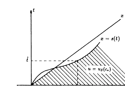
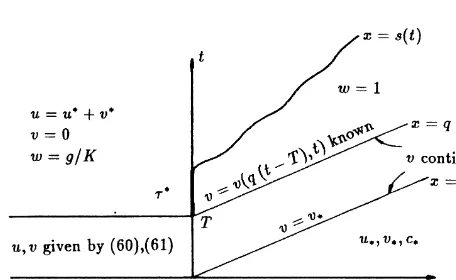
The mathematical argument is the following. Suppose the dissolution front moves ahead of the fluid front, as in Fig. 1. Since w(x,t)¼1 for x.s(t) we find from eqn (21) that u¼
uS(c*) in the shaded region in Fig. 1. Next select tˆ.0 such
that
s(ˆt).qˆt ands˙(ˆt).q (24)
where the dot denotes differentiation. In other words, we have selected a time tˆ at which the speed of the dissolution front exceeds q. Then by the Rankine–Hugoniot condition (eqn (22)),
u(s(tˆ)¹,ˆt).up¼uS(cp) (25) as v jumps downwards from right to left or does not jump.
Here u(y¹,t)¼limx↑yu(x,t) denotes the limit in y from the left and u(yþ,t)¼limx↓yu(x,t) the limit from the right. But
c(s(tˆ),tˆ)¼c*and thus by eqns (3) and (20) u(s(ˆt)¹,ˆt)#uS(c
p) (26)
a contradiction. In other words, eqn (24) implies over-saturation for u. But this is not allowed under equilibrium conditions. We further note that if v is discontinuous at the dissolution front, i.e. v(s(t)þ,t) . 0 then s˙(t) ¼ q cannot
occur. This is a direct consequence of eqn (22). This obser-vation implies that s(tˆ)¼qtˆ and s˙(tˆ)¼q for some tˆ.0 can
also not occur as v(s(tˆ)þ,tˆ)¼v*. 0. Hence
s(t),qt for all t.0 (27)
The ordering of the fronts and eqns (20) and (21) imply
u(x,t)¼
#uS(cp) ¹` ,x,s(t)
uS(cp) s(t),x,qt
uS(cp) qt,x, þ`
8
> > <
> > :
(28)
Consequently by eqn (22)
0#s˙(t)#q for all t.0 (29)
and s˙(tˆ),q occurs at points tˆ where v is discontinuous. In
paxticular this shows that all dissolution fronts are mono-tone in time. Since v vanishes in the region x, s(t), we
have there
]u ]tþq
]u
]x¼0 (30)
The initial condition on u for x,0, the upperbound in eqns (29) and (30) imply that u¼u*for x,s(t). To determine v
in the region x.s(t) we use eqns (15) and (28). Combined,
they imply that ]v(x,t)/]t ¼ 0 for x . s(t), x Þ qt. Then
using the initial condition on v for x . 0 and the lower bound on s˙, we find after integration v¼v*, for x . s(t).
Thus we have constructed a piecewise constant solution of eqns (3), (15) and (20) which satisfies the initial distribution (eqn (7)). The dissolution front follows from the Rankine– Hugoniot condition (eqn (22)): s(t)¼at, with
a¼ uS(c p)¹up
uS(cp)¹upþvp
q(,q) (31)
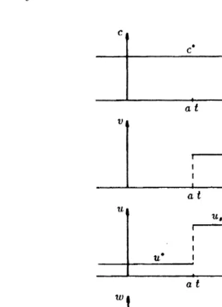
Across the other shock, x¼qt, v is constant. This is
con-sistent with eqn (22). In the chemical engineering literature this front is called the salinity front, see e.g. Bryant et al.1). In Fig. 2 we show the level set of the solution {u, v, w, c} at equilibrium. The separating curves are shock curves at x¼at
and x¼qt. Fig. 3 shows a sketch of the profiles of the
vaxi-ables for some t.0. A qualitative comparison with the
com-putations of Willis and Rubin15will be given in Section 5. One may raise the question if the solution as constructed in this section is the unique solution of the initial value problem. For the following reasons we believe that it is. In the construction, inequalities (eqn (29)) are crucial. They imply directly that the concentrations u and v are constant to the left and the right of a dissolution front, lead-ing to the constant speed eqn (31). In eqn (29) the inequal-ities are a consequence of the Rankine–Hugoniot condition and the fact that oversaturation is ruled out by requiring w,1 in eqn (3). In other words, eqn (29) exhibits local properties of any dissolution front. As outlined above they lead to a piecewise constant solution as presented in this section.
3 NON-EQUILIBRIUM
When precipitation–dissolution reactions cannot assumed to be at equilibrium, one needs to incorporate the first-order reaction eqn (2) in the description. This leads to a much more involved analysis. In this section we construct solutions of the Riemann problem (eqns (2)–(4), (7) and (15)) for two distinct cases. In Section 3.1 we assume eqn (10) to be satisfied, implying that crystalline solid is present only in part of the flow domain, and in Section 3.2 we assume v*, v* . 0. In this first case a dissolution front
exists for all t $ 0. In the second case it may appear in
finite time.
3.1 Crystalline solid partly present
Inspired by the equilibrium results, i.e. ‘k ¼ `’, we start with the assumption that a dissolution front exists, as in eqn Fig. 2. Level sets of concentrations at equilibrium.
(23), which satisfies inequalities eqn (29). These inequal-ities are crucial for the construction of a solution. Unfortu-nately there are no obvious physical or mathematical axguments to support these assumptions. In contrast, the weaker statement s(t)#qt for all t$0, which is obviously
physical, can be justified similarly as in Section 2. We return to the possibility of existence of solutions not fulfilling these assumptions when discussing the uniqueness at the end of Section 4. The main goal is to derive an equation for the location x¼s(t) of the dissolution front.
As in Section 2 we conclude, because of
(]v=]t)¼0 for x,s(t), that u ¼ const ¼ u* for x , s(t)
and that w ¼ g(u*, c*)/K there. Similarly for x . qt we
have u¼ const¼ u* ¼ uS(c*) and thus v ¼const ¼v*.
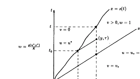
With reference to Fig. 4, we are going to consider the fol-lowing problem:
Note that in the composite solution the crystalline concen-tration v is continuous across x¼qt, due to eqn (22) and
then eqn (35) holds, while the fluid concentration u possibly has a discontinuity there. Eqn (33) implies continuity of v across the dissolution front x¼s(t), which in turn, due to
eqn (22), implies continuity of u across x¼s(t).
We solve eqns (32) and (33) by the method of character-istics. Choose any point (y,t) in the domain {(x,t):s(t),x, qt, t.0}, see also Fig. 4. The characteristics of eqn (32) are
straight lines in the (x,t)-plane, having slope q with respect to the t-axis. The characteristic passing through the point (y,t), i.e. the curve x¼yþq(t¹t), intersects the dissolu-tion front in the point (s(t0), t0), which satisfies
s(t0)¼yþq(t0¹t) (36)
Due to s˙(t)#q this point is unique and thus is the same for
all starting points (y,t) satisfying eqn (36). For a given dissolution front s(t), this would determine t0as a function
of y andt, i.e. t0¼t0(y,t).
Integrating eqn (32) along the characteristic and using eqn (36) yields
The idea is now to use eqn (33) and the boundary condi-tions on v to determine the location of the dissolution front, i.e. to find the function s(t). Before we proceed we first introduce for the case u*, uS(c*) the functionƒ:[0,þ`)
characteristic from the dissolution front x¼s(t0) to a point (y,t), whileƒ(d)¼u(y,t) denotes the fluid concentration at that point. The fluid concentrationƒ and reaction rate F at any point of a characteristic depend only on this distanced, which is due to the fact that convection is the only transport mechanism in this single reaction problem. Note that due to the differentiability of g(.;c*) at u¼uS(c*)
Zu
up
1
k{K¹g(z; cp)}dz→`for u →uS(cp) (40) and thusƒand F are well defined.
Examples. Let the rate function g be given by the law of
mass action (eqn (11)). We can explicitly compute the cases:
We find thatƒsatisfies
where
uS¼uS(c),u0¼u0(c)¼
c
2¹ 1 2
c2þ4K
p
anda¼k
q(uS¹u0)
Consequently
F(d)¼k(uS¹u0)
2up ¹u0
uS¹up
e¹ad
e¹adþup ¹u0
uS¹up
2 (44)
When u*¼uS(c*), which we consider as a degenerate case,
we extend the definitions (eqns (38) and (39)) by setting
f(d)¼uS(cp)and F(d)¼0 for alld$0 (45)
Unless stated otherwise we avoid this degeneracy by taking
u*, uS(c*). This implies F(d). 0 and F9(d),0 for all d$ 0.
Next we continue the analysis of eqns (32) and (33), by rewriting eqn (37). Take any t.0 and let y ¼s(t). Using
eqns (38) and (39) we now write
k{K¹g(u(s(t),t); cp)}¼F(s(t)¹s(t
0)) (46)
for any s(t)/q,t,t. Here we have used s˙(t)$0. In this expression, t0¼t0(s(t),t) satisfies t0¼t whent¼t.
Sub-stituting eqn (46) into eqn (33), integrating the result in time and applying the v-boundary condition in eqns (34) and (35), yields
Zt
s(t) q
F(s(t)¹s(t0))dt¼vp (47)
Note that in deriving this equation we in particular assumed
s to be monotone, but not to be strictly monotone. In the
derivation of eqn (47) we can allow for constant parts of s, i.e. for times 0#t,t2such that s(t)¼s(t1) for all t1#t# t2. In such a case the definition of t0¼t0(s(t),t) gives for t
such that t1#t #t2:
t0(s(t),t)¼tfor t[[t1,t] (48)
and the whole derivation of eqn (47) holds true with the following exception: if s(t) ¼0 for 0 # t # t2, then the
integration leading to eqn (47) cannot be performed for t[
[0,t2] as v(0,0) is not defined. But on the other hand a
dissolution front as sketched in Fig. 4, i.e. s(0) ¼ 0 and
s(t).0 for t.0, would lead to a contradiction in eqn (47). Letting t↓0 would make the left hand side zero while v*.0
as given. Therefore, we have a waiting time t*.0, see Fig.
6, such that
s(t)¼ 0 for 0
#t#t
p,
.0 for t.t
p (
(49)
From eqn (47) for t↓t*, we conclude
tpF(0)¼vp (50)
Using eqns (38) and (39) we find for the waiting time the expression
tp¼ vp
k{K¹g(up,cp)} (51)
Note that in the degenerate case u* ¼ uS(c*) eqn (51)
implies t*¼`. In other words, when u*equals the
solubi-lity concentration then the dissolution front remains stag-nant. Furthermore, apart from the initial waiting time, no further constant parts of s can occur: if this would be the case, say on the interval [t1,t2], then we conclude from
eqn (47)
vp¼
Zt2
s(t2)=q
F(s(t2)¹s(t0))dt (52)
¼
Zt2
t1F(s(t1)¹s(t0))dtþ
Zt1
s(t1)=qF(s(t1)¹s(t0))dt
¼
Zt2
t1
F(0)dtþvp,
which is a contradiction. We want to rewrite the integral in eqn (47) in terms of t0and we do this by using eqn (36).
From that equality, with y¼s(t), we obtain due to s˙(t)#q
a unique correspondence of the pointstwith the points t0,
where
t: s(t)
q →t implies t0: 0→t
and
]t
]t0¼1¹
1
qs˙(t0) (54)
Fig. 5. Rate function g for n¼m¼1. Note that u*$c.
Applying these observations to eqn (47) yields
where the left-hand side can be slightly rewritten by intro-ducing the waiting time:
To summarize, we have obtained an integral equation from which the location of the dissolution front can be deter-mined. The precise formulation is: Let t*be given by eqn
(51). Then find the function s(t), satisfying eqn (49) and the dissolution front equation (DFE)
The expression for B follows from eqns (50), (55) and (56). In general we have to rely on numerical methods to solve (DFE). One such method will be discussed in Section 5. Only very special cases can be solved analytically, for instance the case n ¼ 1 and m ¼ 0 (the linear case) in the examples, where F is given by eqn (42). For that form of F it is straightforward to solve (DFE) explicitly. The result is
In Section 4 we show how to transform (DFE) into a standard integral equation, from which some characteristic properties of the front can be derived. Having found an expression or approximation for s(t), one has to go back to eqns (37) and (38) to determine u. The concentration of the crystalline solid is obtained from integrating eqn (33).
3.2 Solid present everywhere
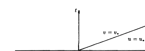
As in the previous case, the concentrations ahead of the fluid front are not affected by the displacing fluid and, therefore, equal to the initial concentrations. Since v is continuous across x ¼ qt, the essential parameters which determine
the behavior of the concentrations are u*, v*, c* (rather
uS(c*)) and v*, see Fig. 7. For definiteness we assume here
that v*,v*. As long as v.0, implying w¼1, no
dissolu-tion front will emerge and we need to solve eqns (32) and
(33) subject to the conditions shown in Fig. 7. From the physical point of view the initial conditions for x, 0 are
somewhat unrealistic because u* and v*are not in equili-brium. This implies that in a laboratory experiment the resi-dent fluid in the region x , 0 at t ¼ 0 has to be
instantaneously replaced by fluid with concentration
u*.The latter is, by approximation, only feasible for (very) small reaction rates.
Integrating the u-equation along the characteristic x¹qt¼ constant and the v-equation in t, we find that
u(x,t)¼ƒ(qt)for x,0 or 0,x,qt and t.0 (60)
withƒdefined by eqn (38) and
v(x,t)¼ v
pþup¹ƒ(qt) for x,0,t.0
vpþƒ(x)¹ƒ(qt) for 0,x,qt,t.0
(
(61)
The latter follows immediately from integration of
]v(x,t) ]t ¼ ¹
]u(x¹qt,t)
]t (62)
in time, see eqn (15). Note thatƒis monotonically increas-ing fromƒ(0)¼u*towards ƒ(`)¼uS(c*). The solid
con-centration for fixed t.0 is sketched in Fig. 8.
Obviously, eqns (60) and (61) are only meaningful if v.0.
This leads us to consider the following cases.
1. u*¼uS(c*).
This choice impliesƒ¼constant¼u*, yielding the solution Fig. 7. Initial conditions for the domain x,qt,t.0.
2. u*,uS(c*) and v*$uS(c*)¹u*.
The second inequality being strict means that the concentration of crystalline solid is too high to be fully dissolved in the fluid. As a consequence eqns (60) and (61) hold for all t. 0, where
Now the second inequality and eqn (61) imply that there exists a finite time T. 0, defined by
ƒ(qT)¼vpþup, (66)
The distribution of the concentrations in the (x,t)-plane is sketched in Fig. 9. At the point (0,T) a dissolution front emerges as explained in Section 3.1, except that the constant
v has to be replaced by the known function v(q(t¹T),t).
Translating the point (0,T) to the origin by setting x¼x,t¼
t ¹T, and writing s¼ s(t) (with s(0) ¼0, s(t) $ 0, for t.0) we find the waiting timet*
tpF˜(0)¼vp¹vp (68) and the modified dissolution front equation (MDFE)
(MDFE)
In the expressions, the function differs from the function
F used in (DFE): obviously u* has to be substituted by
ƒ(qT)¼u*þv*in the definition of a function f˜ in eqn (38) and F is given by eqn (39) by substitutingƒby f˜. Further-more, the function V in B˜ is related to v along x¼q(t¹T). It Note that here the original functionƒaccording to eqn (38) appears in eqn (71). Clearly V(0)¼0. Having determined
s(t) from eqn (68), (MDFE) and eqn (71), one proceeds as before to find u and v in the region s(t), x, qt,t. 0.
In principle a discontinuity of u is possible at x¼q(t¹T).
In fact u is continuous there, which can be seen as follows: due to eqn (60) we have u(q(t¹T)þ,t)¼ƒ(qt)¼ƒ(xþqT). On the
The qualitative analysis concerning dissolution fronts, as given in Section 4, is restricted to (DFE) only. This choice implies no loss of generality. All results/properties carry over to the solution of (MDFE). However, when discussing the numerical results, we do present an example in which a con-centration distribution as shown in Fig. 9 will arise.
4 DISSOLUTION FRONT EQUATION
Before discussing the qualitative behavior of the dissolution front, i.e. the solution of integral equation (DFE), we recall here that this equation was derived by assuming the struc-tural conditions (eqn (29)). These conditions are consistent with the following results.
Proof.
(1) By assumption, s(t)$0 for all t$t*. Since F9(d),0
for alld$0, with F(0)¼k{K¹g(u*;c*)}.0 and F(`)¼0,
we observe that the expression B in (DFE) has the property
B(0)¼0, B(x). 0 for x. 0. Evaluating (DFE) at t¼t*
yields B(s(t*))¼0, implying at once s(t*)¼0.
(2) Differentiating (DFE) with respect to t and rearran-ging terms yields
gives the desired result*.
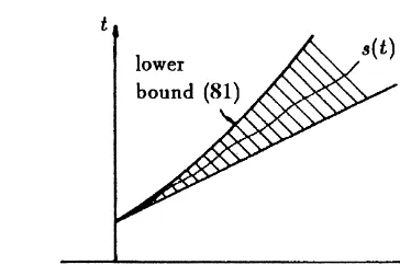
(3) Because the right hand side in eqn (75) is strictly positive, the lower bound is immediate. The upperbound is more involved. To show it we argue by contradiction. Thus suppose there exists t˜.t*such that
˙
s(t),q for all t
p#t,˜t and s˙(t˜)¼q: (76) Taking t¼t˜ in eqn (75) and estimating
¹
This contradicts eqn (76) and, therefore, s˙(t) , q for all t$t*.
(4) To prove this we construct a lower bound which becomes unbounded as t→`. Let
This shows that s(t) becomes unbounded as t→`, see also
Fig. 10.
Having determined these a priori properties of the disso-lution front, we now turn to the question of existence. To make use of well-known results, we transform the equation to a standard linear integral equation of the second kind for a new unknown function. Due to monotonicity Property (3), by a change of variable (see the line below eqn (88)) , we
can rewrite (DFE) as a linear integral equation of the first kind for the derivative of the inverse of s, denoted by f. By differentiation with respect to t, this equation transforms to
B9(x)¼F(0)f(x)þ
Zx
0F
9(x¹y)f(y)dy for x$0 (82)
where the primes denote differentiation and where B and F are as in (DFE). In particular
B9(x)¼1
qF(x)¹tpF9(x) (83)
Eqn (82) has been studied in the mathematics literature and it is known that if F[Hloc1 ([0,`))(i.e. F and F9are locally
square integrable on [0,`)) then eqn (82) has a unique
global solutionfon [0,`), see Zabreyko and Mayorova17.
Furthermore, if F is continuously differentiable (in fact F belongs to C` in many relevant examples) then f is con-tinuous (or also C`) in [0,`). As in the proof of (3), one
easily finds
f(x). 1
qfor all x$0 (84)
Having established the existence of a smooth function f
satisfying eqns (82) and (84), we are now in the position to define the function s: [0,`) → [0,`) such that s(t) ¼ 0
continuously differentiable satisfying (3). Thus s is strictly increasing for t$t*and also s(`)¼`holds true due to the
absence of singularities inf. In this way, there is a one-to-one correspondence of the points x$0 and s(t) for t$t*.
Writing
In the last equality we used the variable transformation
s¹1(y)→t0, as due to eqn (85) we have d/dy(s
¹1
(y))¼f(y). This proves the existence of a continuously differentiable dissolution front for t$t*which satisfies (DFE).
We conclude this section with a remark about uniqueness. Any solution of the Riemann problem eqns (2)–(4), (7) and (15), for which a dissolution front x¼s(t) according to eqn
(23) exists must be of the form discussed in Section 3 with s satisfying (DFE), provided that eqn (29) is satisfied. Now suppose two solutions are possible. They would satisfy Property (3) and thus, using eqn (85), one could define two solutions to the integral eqn (82). But eqn (82) has only one solution which yields a contradiction. The question arises if solutions are possible with dissolution fronts violat-ing eqn (29). If a solution is such that the violation occurs only after some time, i.e. there is a t1.0 such that
0#s˙(t)#q for 0#t#t1 and˙s(t1)¼0 ors˙(t1)¼q
(89)
then s satisfies the integral equation eqn (47) in the interval [0,t1] and the waiting time t*according to eqn (51) exists.
Assume that t1 . t*. Then the integral equation (DFE) is
valid in [t*, t1] and Property (3) implies 0,s˙(t1),q, i.e. a
contradiction. Thus the only possible further solutions we cannot exclude at the moment have the very unlikely prop-erty that there are points tˆ arbitrary close to t¼0 such that s˙(tˆ),0 or s˙(tˆ). q.
One should bear in mind that not every uniqueness con-dition is an entropy concon-dition, i.e. a concon-dition which selects from all possible solutions a physical solution. One should also understand that the differential equation describing the dissolution process, has a smoothing effect on the solution. Discontinuities do not occur at the dissolution front, but only at the known front x ¼ qt. Therefore, interpreting
eqn (22) in terms of ‘entropy’ is misleading. Van Duijn and Knabner4 analyzed in full detail the traveling waves when diffusion is present in the model: the so called visc-osity solutions. As solutions are continuous across the dis-solution front, no information concerning eqn (22) is to be gained from that analysis.
5 NUMERICAL METHOD AND RESULTS
In this section we construct numerical solutions of the Rie-mann problem eqns (2)–(4), (7) and (15). The numerical solution procedure is based on the method of characteristics
and follows the lines of Section 3 in detail. We shall give quantitative results for two distinct non-equilibrium cases:
1. The crystalline solid is only present in the flow domain where x. 0, i.e. v*¼0, v*. 0
2. The crystalline solid is initially present everywhere in the flow domain, i.e. v*, v*.0
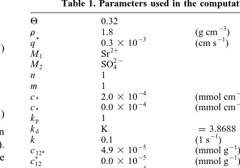
The parameters used in the computations are adopted from Willis and Rubin15and listed in Table 1. The differ-ences are the following: K is slightly larger, in Willis and Rubin15only the equilibrium case k¼`is considered. K is
determined by c1*and c2*and thus has to be different from
Willis and Rubin15, as we do not consider Debye–Hu¨ckel corrections in our computations. But note that also these could be handled without problems as the rate function is of general form. The value of fluid concentration cp1used in
our computations differs from the value given in the caption of Fig. 3 in Willis and Rubin15. The value in the caption is
cp
1 ¼(Sr2
þ
)f¼2.0310
¹5mMol cm¹3(which we used in
Ref.7) while Fig. 3 suggests that the correct value used by Willis and Rubin 15 equals cp
1 ¼ 2.03 10
¹4mMol cm¹3.
We decided to use the latter value in this paper.
5.1 Numerical method
The numerical procedure consists of the following steps: evaluation of integral (eqn (38)) to obtain a numerical approximation of the function ƒ(d), substitution of ƒ(d) in eqn (39) to obtain F(d), numerically solving a Volterra inte-gral equation which follows from (DFE) to find the location of the dissolution front s(t) and finally we go back to eqns (37) and (38) to determine u. The concentration of the crys-talline solid is obtained by integration of eqn (33).
The integrand of eqn (38) becomes singular when u*
tends to the solubility concentration us(c*). This singularity
has to be handled with care because we need numerical approximations of f(d) in a wide range of d values. We used Clenshaw–Curtis quadrature in combination with sym-bolic transformation techniques to remove the singularity, as implemented in the computer algebra system Maple, see
Table 1. Parameters used in the computations.
Geddes5. The result of the numerical integration is given as a table [di,ƒ(di))], wheredi¼i·Dd. Only in special cases, i.e.
n ¼ 1, m ¼ 0 (the linear case) and n ¼ m ¼ 1, exact evaluation of integral (eqn (38)) is possible. We used the exact eqns (41) and (44) to verify the accuracy of the numer-ical integration of eqn (38). The discrete result of eqn (38) is used to evaluate eqn (39), i.e. F(di) on thed-grid.
Eqns (82) and (83) can be written as a standard linear Volterra integral equation of the first kind, i.e.
t(d)¼h(d)¹
Zd
0K(d¹y)t(y)dy (90)
where
h(d)¼1
q F(d) F(0)¹tp
F9(d)
F(0) (91)
and kernel
K(d¹y)¼F9(d¹y)
F(0) (92)
We solve this equation explicitly, using the trapezoidal rule to discretize the integral in eqn (90). The approximation of the derivatives are chosen central in d, except in the first integration step where the derivatives are discretized forward ind. The position of the dissolution front follows from the definition of r, hence
t¹tp¼
Zs(t)
0 t(z)dz (93)
Becausetis computed at the location of the grid points we have s(t)¼iDdand the corresponding value of t is found by approximating the right hand side of eqn (93) using Simp-son’s rule. To compute a profile of the fluid concentration u at a certain time level t1 we choose a point P(y,t1) in the
(x,t)-plane (see Fig. 11). We walk backwards along the characteristic through point P and compute the coordinates of the intersection point (s(t0),t0) of the characteristic and
the free boundary curve s(t). The precise procedure is as follows: start in point P, follow the characteristic in the direction of the dissolution front s(t), check in every grid point if the t-coordinate of the characteristic is above the corresponding t-coordinate of s(t) in that point. If this is the case we use the last and before last step to compute the
intersection point of the characteristic and s(t), assuming that the approximation of s(t) is piecewise linear between successive coordinates. This gives the desired value
dt1¼y¹s(t0), corresponding to point P. Next we use the table of discrete [di,ƒ(di)]-values to compute the fluid con-centration u(y,t1)¼f(dt1) in P. Because dti (usually) does not coincide with one of thedi-values in the table, we have to interpolate once more. A fluid concentration profile is constructed by repeating this procedure in the region
s(t1) # y # q(t1¹t*) at a sufficiently large number of
points P.
To obtain a numerical approximation of the concentration v of the crystalline solid in point P(y,t1) we first have to
obtain values of the fluid concentration in discrete points along the vertical line through (y,t2) and (y,t1) using the
procedure given above, see line B in Fig. 11. By explicit integration in time of eqn (33) from the position of the free boundary, i.e. t2, to the position of P, i.e. t1, we obtain v(y,t1).
Full integration from the position of the free boundary (s(t2),t2) to the position of the fluid front (y,t3) has to
repro-duce the boundary condition v*(up to a small error, due to
the discrete numerical approximations), which follows from eqn (47). This serves as a check for the accuracy of the numerical procedure. For the linear case (n ¼ 1, m ¼ 0) we compared results obtained by the numerical procedure and the corresponding exact solutions and found excellent agreement.
5.2 Results
In this section we give computed results for the following cases:
1. The linear case n¼1, m¼0 for v*¼0
2. A non-linear case n¼1, m¼1 for v*¼0 and for v*,
v*.0
3. A non-linear case n¼2, m¼2 for v*¼0.
Remark. In order to obtain comparable time, space and
concentration scales for all cases considered in this section we introduce an artificial factor a that multiplies the func-tion g and assume K¼3.8688310¹7to be independent of the values of n and m. This implies that only the results of the computations for the case n ¼ m ¼ 1 have physical meaning. The values of a used in the computations are: .
n m a
1 0 6.22310¹4
1 1 1.0
2 2 1.83310þ6
5.2.1 The linear case: n¼1, m¼0
Fig. 12 shows the position of the crystal dissolution front in the (x,t)-plane for the linear case (n ¼ 1, m¼0). In this example we have t*¼10499 s. The dissolution front is a
straight line which satisfies exactly eqn (58). Due to the introduction of a we have to replace kt* by akt* in the
denominator of eqn (58). Fig. 13 shows breakthrough curves of the fluid concentration at different observation points. An observation independent of this special case is: There are horizontal parts in these curves, which correspond to the fluid concentration in the region in the (x,t)-plane where
x1/q # t # x1/q þ t* at a given position x ¼ x1. In this
regiond¼x1is constant and, therefore, u is constant, u¼
ƒ(x1) increasing monotonically from u* to uS(c*) for x1
ranging from 0 to `. The width of the flat region in all
curves is constant and equal to the waiting time t*. Fig. 14
shows the time evolution of the crystalline solid concentra-tion at different posiconcentra-tions. The regions with constant slope in the v-curves correspond to the regions in the breakthrough curves for u where u is constant.
Fig. 15 gives profiles of the fluid concentration at different time levels. We observe several points in the u-profiles where the derivative ux¼]u/]x is discontinuous. The discontinuity in uxat the toe of the profiles in Fig. 15 travels with speed s˙(t). A simple computation shows that for the general case
]
]xu(s(t)
þ,t)¼k{K¹g(up; cp)} 1
q¹s9(t¹) (94)
The second discontinuity (from the left) in uxreflects the discontinuity of s˙(t) at t ¼ t*. Its position is a point at
the line x ¼q(t¹t*) in the (x,t)-plane for a given time t.
In fact, we have in general due to Property (2) for such (x,t)
]
]xu(x þ,
t)¹ ]
]xu(x ¹,
t)¼ ¹f9(x) 1 ktp ]
]ug(u
p; cp) (95)
At the fluid front, i.e. the top of the u-profile, we have a jump in u which is consistent with the Rankine–Hugoniot shock condition eqn (22), and given by
u(qtþ,t)¹u(qt¹,t)¼up¹ƒ(qt)→up¹uS(cp),0
(96)
An exception is the linear case, as here uS(cp)¼uS(c*)¼ u*and thus the discontinuity at x¼qt vanishes for x1→`.
Fig. 16 shows the corresponding profiles of v. The deriva-tive vx¼]v/]x at the dissolution front is discontinuous, due
to the discontinuity in u at the front. The constant speed is Fig. 12. Dissolution front in the (x,t)-plane for the linear case.
Fig. 13. Breakthrough curves of the fluid concentration u at
dif-ferent positions for the linear case. From left to right the observa-tion points are: x¼2, 6, 10, 14, 18, 22, 26 and 30 cm (see Fig. 12).
Fig. 14. Time evolution of the crystalline solid concentration v at
different positions for the linear case. From left to right the observation points are: x ¼ 2, 6, 10, 14, 18, 22, 26 and 30 cm
(see Fig. 12)
Fig. 15. Fluid concentration profiles at different time levels for the
given according to eqn (58) by
˙
s(t)¼ q 1þktp¼
up¹u p
up¹u
pþvp¹vp
q (97)
which corresponds to the speed of travelling waves, which exist for constant c [compare Ref.7, in particular equation
(54)]. By inspection of the explicit solution given by eqns (36), (41), (59) and (97) for the Riemann problem and the explicit solution for the travelling wave problem (note that
g is independent of c here, see e.g. the first example in
Section 3.1) derived from Ref. 7, eqns (54) and (93) we see that for taking the shift L¼at*, where a is given by eqn
(97), the solutions coincide for x , (t¹t*)q. In particular
there is pointwise convergence in x for t→`of the
solu-tion profile here to the travelling wave solusolu-tion.
5.2.2 A non-linear case: n¼1, m¼1
For this case we shall distinguish between the two sets of initial and boundary conditions as discussed in Sections 3.1 and 3.2.
5.2.3 Solid only partly present (See Section 3.1)
In this case the solubility concentration is given by
uS(c)¼c=2þ1=2
c2þ4K
p
, i.e. uS(c*) . uS(c*) ¼ u*.
We have chosen c* ¼u* ¼2.0 3 10-4. Because c* ¼0
we now have K ¼u*(u*¹c*) ¼ u
2
p, see Table 1. For the waiting time t*we find 7108.0 s. The dissolution front s(t) is
now a curve with slope s˙,q for all t$0. Fig. 17 shows the
position of the dissolution front in the (t,x)-plane. The curve suggests that s˙(t*)¼ q which is not true. In fact the s˙(t*)
satisfies Property (2) in Section 4 where in this example it turns out that F9(0)1F(0)t*q , 1. Fig. 18 shows
break-through curves of u for different observation points. The qualitative differences as compared to the linear case are the following: (1) the toe of the u-profile does not travel with constant speed but with speed s˙(t). (2) After a certain time the maximum concentration in the profiles exceeds u*and
increases in time to the solubility concentration uS(c*). (3)
The fluid concentration at the fluid front remains discontin-uous and jumps either from below or from above to u*.
Fig. 19 gives the corresponding curves for v. The properties of the time evolution of the crystalline solid concentration compare to the those in the linear case, see Figs 14, and 19. Fig. 20 shows the fluid concentration profiles at different Fig. 16. Crystalline solid concentration profiles at different time
levels for the linear case. From left to right the curves correspond to t¼20 000, 40 000, 60 000, 80 000, 100 000 s (see Fig. 12)
Fig. 17. Dissolution front in the (x,t)-plane for the non-linear case
n¼m¼1.
Fig. 18. Breakthrough curves of the fluid concentration at
differ-ent positions for the non-linear case n¼m¼1. The observation points are x¼3.0, 6.0,…, 18.0 cm (see Fig. 17)
Fig. 19. Time evolution of the crystalline solid concentration at
time levels for the non-linear case. The corresponding crystalline solid concentrations are given in Fig. 21.
A quantitative comparison between the solutions of the Riemann problem for the non-linear case and the solutions found by Willis and Rubin15is not possible because they allow for diffusion in their problem and consider only equi-librium reaction. Comparing Fig. 3, Fig. 20 and the corre-sponding general statements mentioned and Fig. 3 of Willis and Rubin 15 indicates: the common qualitative property caused by the interplay of transport and dissolution is a ‘plateau-structure’, which for a fixed time t is defined by the spatial intervals I1¼{xlx,s(t)}, I2¼{xls(t),x,qt}, I3¼{xlx. q)}. In I3the solution is given by the ‘initial
condition’ u* ¼uS(c*), in I1by the ‘boundary condition’ u*¼uS(c*) and in I2at least asymptotically, i.e. for large t,
by uS(c*). The piecewise constant structure of Fig. 3 without
dispersion and kinetics is smeared out by the addition mechanisms in different ways. Kinetics leads to a smooth-ing effect in I2such that the transition at x¼s(t) becomes
continuous and the maximum is attained at x¼qt. Diffusion
smooths more, effecting also I1and I3and leading to overall
smooth and nonconstant profiles, where the maximum in I2
is attained at x¼s(t). The solutions for other values of n and m have properties that compare to the solutions of the
non-linear example discussed in this section.
5.2.4 Crystalline solid present everywhere. (See Section 3.2)
Two characteristic times arise in this case: T ¼ 2680 s, which is the time needed to dissolve all initially present crystalline solid (v* ¼ 1.0 3 10¹4) in the region x , 0 andt*¼4903 s, which is the waiting time for the
dissolu-tion front. For t$T we have u¼u*þv*¼3.0310¹4in
the region x,0. Fig. 22 shows the position of the
dissolu-tion front in the (x,t)-plane. Fig. 23 gives breakthrough curves of u and the time evolution of v at different positions in one graph. The upper set of curves is u and the lower is v. The horizontal parts in the u-curves have widtht*and give rise to linear parts in the v-curves, while the increasing parts, which vanish as time proceeds, have width T. The Fig. 20. Fluid concentration profiles at different time levels for the
non-linear case n¼ m¼1. From left to right the curves corre-spond to t¼10 000.0, 20 000.0,…, 60 000.0 s (see Fig. 17).
Fig. 21. Crystalline solid concentration profiles at different time
levels for the non-linear case n¼ m¼1. From left to right the curves correspond to t ¼ 10 000.0, 20 000.0,…, 60 000.0 s (see
Fig. 17).
Fig. 22. Dissolution front in the (x,t)-plane for the case n¼m¼1 v*, v*.0 (compare with Fig. 9).
Fig. 23. Breakthrough curves of u (upper curves) and time
crystalline solid concentration along the line x¼q(t¹T) in
the (x,t)-plane is known and given by eqn (61). We used this to check the accuracy of the computations.
5.2.5 A non-linear case: n¼2, m¼2
For any combination of n, m $ 1 the function g(u;c*) is monotonically increasing and convex in the interval (c/m)
#u#uS(c*) and, therefore, we may expect similar
quali-tative behavior of the solutions. The position of the dissolu-tion front in the (x,t)-plane is shown in Fig. 24. Now the solubility concentration is given by
uS(c)¼
c
4þ 1 4
c2þ16pK=a
q
The factor a is chosen such that uS(c)¼7.299310
¹4, as in
the case n¼m¼1. The breakthrough curves of u are given in Fig. 25 and the corresponding time evolution of v in Fig. 26.
6 CONCLUSIONS
We considered a model for transport and dissolution– precipitation, where the kinetics of the reaction is taken into account, but diffusion–dispersion is ignored. The appearance and evolution of a dissolution front from corre-sponding initial states, i.e. the Riemann problem of the hyperbolic system, is investigated. The initial states for the ‘charge distribution’ c are ‘incompatible’ in general, i.e. the ‘ionic composition’ of the fluid changes. The method of characteristics leads to a nearly explicit representation of the solution, where only an implicitly defined functionƒeqn (38) has to be evaluated numerically and based on ƒ an integral (eqn (57)) has to be solved numerically [or rather the transformed eqns (82) and (83)]. The basic ‘plateau-structure’ of the solution is revealed being characterized by the dissolution front x ¼ s(t) with speed less than q,
where (for non-equilibrium) ]u/]x and]v/]x are
discontin-uous and the fluid or salinity front x¼qt, where u and]v/]x
are discontinuous. A comparison of solutions elucidates the role of kinetics and of diffusion–dispersion, which turns out to be similar, but in detail different mechanisms. In addition, due to non-equilibrium, the dissolution front s only starts to move after a positive time t*, with positive slope, which
implies a discontinuity in]u/]x at x¼q(t¹t*). Because of
these properties the solutions are principally different from the travelling wave solutions of Ref. 7 for ‘compatible’ boundary conditions and only local convergence can be expected for t→`.
REFERENCES
1. Bryant, S.L., Schechter, R.S. & Lake, L.W. Mineral sequences in precipitation –dissolution waves. AIChE J., 1987, 33, 1271–1287.
2. Bryant, S.L., Schechter, R.S. & Lake, L.W. Interactions of precipitation –dissolution waves and ion exchange in flow through porous media. AIChE J., 1986, 32(5), 751–764. 3. Dria, M.A., Bryant, L., Schechter, R.S. & Lake, L.W.
Inter-acting precipitation –dissolution waves: the movement of
Fig. 24. Dissolution front in the (x,t)-plane for the case n¼m¼2, v*¼0
Fig. 25. Breakthrough curves of u at x¼3, 6, 9 and 12 cm for the case n¼m¼2, v*¼0.
inorganic contaminants in groundwater. Water Resour. Res., 1987, 23(11), 2076–2090.
4. Van Duijn, C.J. & Knabner, P. Travelling wave behaviour of crystal dissolution in porous media flow. Euro. J. Appl. Math., 1997, 8, 49–72.
5. Geddes, K. O., Numerical Integration in a Symbolical Con-text. In Proceedings of SYMSAC’86, ed. B. Char. ACM Press, New York, 1986, pp. 185–191.
6. Helfferich, F. & Klein, G., Multicomponent Chromato-graphy. Dekker, New York, 1970.
7. Knabner, P., Van Duijn, C.J. & Hengst, S. An analysis of crystal dissolution fronts in flows through porous media. Part 1: compatible boundary conditions. Adv. Water Res., 1995,
18(3), 171–185.
8. LeVeque, R.J., Numerical Methods for Conservation Laws. Birkha¨user, Basel, 1992.
9. Noval, C. F., Lake, L. W. & Schechter, R. S. Geochemical modelling of two-phase flow with interphase mass transfer. AIChE J., 1991, 37(11), 1625–1633.
10. Novak, C. F., Schechter, R. S. & Lake, L. W. Diffusion and solid dissolution–precipitation in permeable media. AIChE J., 1989, 35(7), 1057–1072.
11. Schweich, D., Sardin, M. & Jauzein, M. properties of con-centration waves in presence of nonlinear sorption, precipita-tion–dissolution, and homogeneous reactions 1 fundamental . Wat. Resour. Res., 1993, 29, 723–733.
12. Sevougian, S.D., Lake, L.W. & Schechter, R.S., KGEO-FLOW: A New Reactive Transport Simulator for Sandstone Matrix Acidizing, Society of Petroleum Engineers, Paper (SPE 24780) Februari 1995, pp. 13–19.
13. Sevougian, S.D., Schechter, R.S. & Lake, L.W. Effect of partial local equilibrium on the propagation of precipita-tion–dissolution waves. Ind. Eng. Chem. Res., 1993, 32, 2281–2304.
14. Walsch, M.P., Bryant, S.L., Schechter, R.S. & Lake, W.L., Precipitation and dissolution of solids attending flow through porous media, AIChE J., 30(2) (1984) 317–328.
15. Willis, C. & Rubin, J. Transport of reacting solutes subject to a moving dissolution boundary: numerical methods and solu-tions. Water Resour. Res., 1987, 23, 1561–1574.
16. Whitham, G.B., Linear and Nonlinear Waves. Wiley, New York, 1974.

![table of discrete [dnot coincide with one of thecentrationi,ƒ(di)]-values to compute the fluid con- u(y, t1) ¼ f(dt1) in P](https://thumb-ap.123doks.com/thumbv2/123dok/3171512.1387878/11.709.40.277.366.485/table-discrete-dnot-coincide-thecentrationi-values-compute-uid.webp)

