Large-scale flow of groundwater in Swedish
bedrock. An analytical calculation
G. Rehbinder
a ,* & A. Isaksson
b aDepartment of Civil and Environmental Engineering, The Royal Institute of Technology, S-100 44 Stockholm, Sweden
b
Department of Signals, Sensors and Systems, The Royal Institute of Technology, S-100 44 Stockholm, Sweden
(Received 23 February 1996; revised 14 November 1996; accepted 13 January 1997)
The flow of groundwater in the bedrock, which might jeopardize the possibility of repositing nuclear waste at great depth in the rock, is mainly governed by the large scale properties of the topography. The topography of Sweden is characterized by the Caledonian mountain chain, which runs through a large part of the Scandinavian peninsula, and by regular large ridges and valleys that are almost perpendicular to the mountain chain. The hydraulic conductivity of the bedrock decreases with the depth, and the characteristic length scale of this variation is much less than the length scale of the topography. The result of the analysis, given here exclusively as closed formulae, shows that the flow takes place in the uppermost 500 m of the bedrock, which is approximately the depth of a future repository. The analysis also shows that the residence time of a fluid particle is inversely proportional to the hydraulic gradient and to the ratio between the length scale of the topography and the conductivity. The residence time also depends on the ratio between the lengths that characterize the topography and the variation of the conductivity with depth. The shortest residence time occurs if the repository is located below a valley, and the longest if it is located under a ridge.q1998 Elsevier Science Limited. All rights reserved.
Key words:groundwater flow, nuclear waste, residence time, topography, periodicity, power spectrum.
NOMENCLATURE
.
a,as,ai,a1 amplitudes of topographical waves
a(z1,z2) filter polynomial a(k1,k2) coefficients e(n1,n2) white noise
f characteristic root
g characteristic root
ki coordinate
K0 reference conductivity
K(z) conductivity
Kˆ(z) dimensionless conductivity
L,Li characteristic horizontal lengths
m wave number
ni wave numbers
Ni number of mesh points
R domain in the x–z-plane
s natural coordinate along a streamline
Smn region of support
t time
T residence time
Tˆ dimensionless residence time
~
n flux per unit area
ˆn¼(ny,nz) dimensionless flux per unit area (x,z) coordinate system
Y(n1,n2) discrete Fourier transform
y(k1,k2) elevation of the topography
yr(n1,n2) reduced elevation of the topography
zi variables of z-transform
z0 characteristic vertical length (y,z) dimensionless coordinate system (y0,z0) dimensionless coordinates at a streamline (yr,zr) dimensionless coordinates of a repository
v angle to the latitude
l geometric similarity parameter
m variance
t dimensionless time
f(x,z) hydraulic potential
f0 reference potential
fs boundary potential
fˆ(y,z) dimensionless potential
F(q1,q2) spectrum
qi frequencies of spectrum
q,q1 frequency of topographical waves
Advances in Water Resources21(1998) 509–522
q1998 Elsevier Science Limited All rights reserved. Printed in Great Britain 0309-1708/98/$19.00 + 0.00
PII: S 0 3 0 9 - 1 7 0 8 ( 9 7 ) 0 0 0 0 9 - 2
1 INTRODUCTION
Radioactive waste repositories deep in the bedrock are thought to be acceptable, from the safety point of view, if the rock is mechanically stable and dense. The Fennoscan-dian shield satisfies such demands and consequently deep repositories are being considered in Sweden. Nonetheless it is important to estimate the flux of groundwater and thereby the residence time of a possible contaminated fluid particle, that has been released from the repository.
The flow of the groundwater in an open aquifer, or in the bedrock, is induced by spatial variations of the level of the phreatic surface. The magnitude of the flux per unit area is determined by two factors. The most important one is the conductivity of the rockmass. The other factor is the mag-nitude of the hydraulic gradient. The latter factor is com-posed of two parts, viz. the variations in the level of the phreatic surface and the lateral length scale of the variations. The situation is sketched in Fig. 1, which shows the topo-graphy of a fictitious landscape. The absence of marked peaks is characteristic for the Fennoscandian shield, which has been subjected to several glaciations. If the lateral length scale is small, the hydraulic gradient is large, which means that the flux per unit area is large but concen-trated to the vicinity of the ground surface. If, on the other hand, the length scale is large, the gradient is small, which means that the flux per unit area is small, but non-negligible at great depth. The shape of the phreatic surface is not characterized by one length scale, but by several. However, the largest of these governs the flow at great depth. In the following, all values are given in SI units.
It is not immediately clear how large the governing lateral length scale is, or if there exists more than onegoverning
length scale. The topography is two-dimensional rather than one-dimensional, as Fig. 1 indicates. The situation becomes even more complicated if the local inhomogeneity and ani-sotropy of the conductivity are significant.
Any length scale that may govern the flow must be com-pared with other possible length scales of the problem. Thus the problem can be split in two parts.
1. Identification of the governing lateral length scales.
If the depth of the repository is large, the governing lateral length scale may be of continental size. Since the phreatic surface is two-dimensional, length scales in different directions may differ. A crucial question is how the characteristic lateral length scales can be measured with reasonable effort. It seems likely that the large lateral length scale of the phreatic surface corresponds to that of the topography. A fictitious
phreatic surface, which corresponds to the fictitious topography, is sketched in Fig. 1.
The largest length scale of the topography os Scan-dinavia is characterized by the Caledonian mountain chain. It causes both the surface water and the ground-water to flow westward to the Atlantic and eastward to the Baltic. The elevation trend due to the mountain chain is one-dimensional but non-periodic.
The topography is two-dimensional in general and has a structure that often appears complex. However, fold-ing and faultfold-ing of the bedrock and loose sand and gravel structures of quaternion origin on top of the
bedrock may cause topographical waves. These can
have characteristic directions and wavelengths, that cannot readily be seen on a map. The Swedish topo-graphic database in GIS can be used to identify pos-sible topographical waves. The database covers the entire country, except for the large lakes in the south-ern part. The mesh is quadratic and the mesh width is 500 m. Thus the database contains almost two million elevation figures.
2. The large scale inhomogeneity of the conductivity of the bedrock.
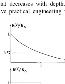
The Fennoscandian shield appears to have at least one large scale hydraulic property. The hydraulic conduc-tivity decreases with increasing depth. The spread of measured data is large, but it has been suggested that the conductivity decreases logarithmically with depth. The simplest representation of such a conductivity, which will be shown to be convenient from a calcula-tional point of view, is:
K(z)¼K0e¹z=z0 m=s (1)
where the z-axis is directed downwards and z0 is a
characteristic length. Carlsson and Olsson2 have
made an extensive investigation of the conductivity at different places in Sweden, particularly in the vicinity of the nuclear power plant at Forsmark. The conductivity was measured with a double-packer per-meameter, meaning thatK(z) may refer to the flow in individual fractures, i.e. to the pore velocity rather than thebulkvelocity. This has an important implication. In the following calculation of the residence time of a fluid particle, the conductivity has notbeen adjusted for the effect of porosity. The implication of this assumption will be discussed. The measurements indi-cated that 50, z0 ,150 and 10-7 ,K0 ,10-5. A
logarithmic decrease of the conductivity is not the only possible representation. The conductivity can also be approximated as a discontinuous function, i.e.,
K(z)¼ K0 0
the characterizations of (1) and (2) is not decisive. Fig. 1.A section of the topography of a fictitious landscape that
Sincekp1, a simple approximation isk¼0. Then an
i.e., the bedrock is effectively homogeneous, but has an impervious bottom.
The two types of conductivities are sketched in Fig. 2. The inevitable small scale inhomogeneity of the conduc-tivity of rock is a serious problem, since it is not covered by the continuum approximation of the large scale. A single crushed zone can serve as a hydraulic ‘short circuit’ that is ignored by the large-scale continuum approximation. It is quite clear that the continuum approximation must be based on the correct length scale, but the smaller the length scale, the higher the demand for correct information about the properties of the rock. Unfortunately, such information is very rarely available.
The residence time of a water particle, particularly a polluted water particle, has been studied theoretically as well as experimentally and articles on the subject are innumerable. The transport of harmful pollutions or harm-less tracers in water that flows through soil or rock is very complicated, since the dispersion, sorption and adsorption depend not only on material properties but on the advection which in turn depends on material properties such as the inhomogeneity.
The inhomogeneity can be tackled using stochastical
methods, as has been shown by Shapiro and Cvetkovic11
and Dagan and Nguyen.3A recent study, which discusses transport and age of groundwater, has been presented by Goode.6
The purpose of the present investigation is threefold. Firstly, to derive closed solutions of the flow equation at very large length scale, i.e., to derive the velocity field, the flow pattern and the residence time of a fluid particle, for groundwater flowing in a permeable half space with conductivity that decreases with depth. Hence, the pur-pose is to derive practical engineering formulae for
geo-hydrologists, so that complicated computer codes can be avoided. Secondly, to present methods by which possible periodic length scales of a given topography can be identified from an elevation database in GIS. Thirdly, to apply the achieved results and formulae to a specific region of Sweden.
2 THEORETICAL ANALYSIS
2.1 Flow of groundwater in the bedrock
An incompressible liquid flows two-dimensionally through a permeable rock that fills a half space. The conductivity and porosity of the rock areK(z) andn, respectively. The equa-tion of the free surface ifz¼fs(x). The amplitude offsis small in the sense thatldfs=dxlp1. The flux per unit area is
called the velocity ~n(x,z). The mass conservation law and Darcy’s law, given by:
=·~n¼0 (4)
~
n¼ ¹K(z)=f (5)
define the flow. K(z) is known. f(x,z) is the unknown hydraulic potential. The boundary condition at the free surface z¼fsis linearized, i.e., the condition is satisfied atz¼0. Thus the real domain,R:{¹` ,x, `,fs#z,
`}, which is shown in Fig. 3(a), is replaced by the fictitious domainRf:{¹` ,x, `, 0#z, `}, which is shown in Fig. 3(b). At infinite depth, the potential is undisturbed. Thus the boundary conditions are:
f(x,z¼0)¼fs(x) (6)
f(x,z→`)¼0 (7)
wherefs(x) is either periodic, or vanishes forlxl→ `. In the latter case f(x) also vanishes for lxl→ `.
As mentioned previously, the conductivity decreases with increasing depth according to eqn (1). Moreover, the shape of the free surface is characterized by a given lengthLand a
given amplitude f0 p L in agreement with the above
assumptions. The length scale L is related to a frequency
q, that is fictitious for the moment. Hence:
q¼2p
L (8)
eqn (1) and (4)–(8) define the problem. Eqn (1), (4), and (5) yield the flow equation
]2f
As Stokes and Thunvik12 pointed out, eqn (1) is the only relationship that yields a closed solution of eqn (9). (z0→` corresponds to constant conductivity.) The terms that contain first-order derivatives are:
Fig. 2.The conductivity of the bedrock as a function of depth. (a) Monotonously varying conductivity, equation (1). (b) Piecewise
1
It is convenient to introduce the following non-dimen-sional variables, including time, and parameters,
ˆ
Three simple cases can be analyzed. They are each two-dimensional, i.e., the topography is characterized by one, or several, regular or irregular, long ridges and valleys.
2.1.1 Simple periodic topography
If the surface potential is simply periodic, i.e.,fˆs(y)¼cosy, the following simple approach
ˆ
f(y,z)¼w(z)cosy, (13)
which goes back to Toth,13 can be used. The method is
described in the textbook by Domenico.4 Introduction of eqn (13) into (12) gives:
d2w
the solution of which is:
w(z)¼ef(l)z (15)
describes the influence of the non homogeneous conductiv-ity. Eqn (13) and (15) give the solution of eqn (12). Hence,
ˆ
The absolute value of the velocity is:
lˆnl¼e(f(l)¹l)zqsin2yþf2cos2y (19)
Equation (18) shows that the greatest absolute value of the vertical velocity occurs below the ‘ridges’ (y ¼0), or the ‘valleys’ (y¼p), whereas the greatest absolute value of the horizontal velocity occurs halfway between a ridge and a valley (y¼p/2), i.e., where the slope is steepest.
The streamlines are given by:
dy=ny¼dz=nz (20)
streamline is uniquely determined byy0.
The velocity and the streamlines offer the possibility of calculating the dimensionless time it takes for a fluid par-ticle to travel between points 1 and 2, along a streamline. Ifs
is the dimensionless natural coordinate, it follows that:
dt¼ds Fig. 3.The flow domain. (a) The real domainR. (b) The simplified
Then: the coordinates of the repository are (yr,zr), the streamline that passes through the repository satisfied:
zr¼ ¹f(l)ln
If point 1 is the location of the repository and point 2
is located at the free surface, i.e., y1 ¼ yr and
If the repository is located below the bottom of a valley, the streamline is vertical and eqn (25) and (27) are not valid. At the vertical streamline, y ¼ yr ¼ y0 ¼ p and ds¼ ¹ dz. The horizontal component of the velocity is equal to zero and:
lˆnl¼fe(f¹l)z; yr¼p, (28)
If the repository is located at very large depth,
lim
Two extreme cases are of practical importance and simple to analyze.
and the streamline through the repository is defined by siny0¼e¹zrsinyr. The equation of the streamline is:
zs¼zrþln
siny
sinyr
(32)
The absolute value of the velocity is thus independent of y, but decreases exponentially with the depth. The time it takes for a fluid particle to travel between points
1 and 2 is:
t2¹t1¼ y2¹y1
siny0
(33)
and the residence time is:
ˆ
T¼e
zr(p¹arcsin(e¹zrsinyr))
sinyr
yrÞ0,p: (34)
If the repository is located exactly below a ridge or a valley, the residence time is
ˆ
Not unexpectedly, the shortest residence time occurs if
yr¼p, i.e., if the repository is located below a valley.
2.l q1
l→`corresponds to a boundary layer solution, since the second order derivatives in eqn (14) vanish. The auxiliary parameters aref< ¹1/landf¹l< ¹l.
The equation of the streamline is:
zs¼
The travel time between two points, 1 and 2, is:
t2¹t1¼
The residence time is:
ˆ
in analogy with the previous case. Similarly, the short-est residence time occurs if the repository is located
below a valley. Since zr,z0, it follows that
infTˆ,e¹1.
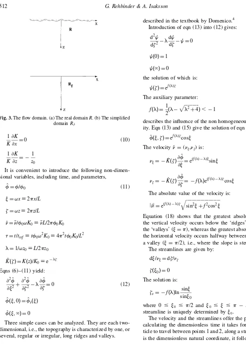
The simplified formulae of the above extremes are sum-marized in Table 1. A comparison between the two extremes shows that increasinglreduces the depth of the streamlines by a factor ofl. This is illustrated in Fig. 4.
If the phreatic surface is periodic in two orthogonal direc-tions, the solution that corresponds to eqn (17) is equally simple. The solution, which is derived in an appendix, might be relevant for a two-dimensional topography that has been created by unstable buoyancy effects. The analysis of this case will not be considered henceforth in this investigation.
2.1.2 Composed periodic topography
In contrast with the previous section, the surface potential contains two terms, viz., the lowest frequency term and a superimposed term, i.e., fˆs(y)¼cosyþa1cosq1y, where q1.1. This case is somewhat more complicated than the
previous one. However, the solution of eqn (12) remains simple. The following approach applies:
ˆ
f(y,z)¼w0(z)cosyþa1w1(z)cosq1y (41)
Eqn (41) is introduced into eqn (12). Algebraic calcula-tions, which are analogous to those presented in Section
2.1.1, yield:
The velocity components are
ny¼e(f0¹l)zsinyþa1q1e(f0¹l)zsinq1y (44)
nz¼ ¹f0e(f0¹l)zcosy¹a1f1e(f1¹l)zcosq
1y
Unfortunately, the equation for the streamlines, eqn (20), cannot be solved in closed form in the general case, but has to be integrated numerically using the method of Runge Kutta, for example. However, iflqq1 .1, the solution
is simple. Hence, the equation of a streamline through (y0,z0) forl qq1, is:
It is not possible to evaluate the integral in eqn (45) in closed form, which is a disappointing shortcoming. Its numerical evaluation is trivial.
The travel time between two points, (y1,z1) and (y2,z2),
is easily evaluated numerically.
The character of the flow pattern, i.e., of the streamlines, depends on the magnitude of the superimposed term. The decisive question is: are there any ‘local ridges and valleys’? i.e., does dfˆs=dy change sign in the interval 0# y # p?
Simple calculations yield that if
a1q21,1 (47)
there are no ‘local ridges and valleys’, and consequently that the flow pattern is dominated by the term that has the lowest frequency. In this case a streamline that has its Fig. 4.Streamlines in a semi-space, that are induced by a simple
periodic topography. (a)l¼0 (homogeneous conductivity), (b)
l¼10 (conductivity decreasing with depth).
Table 1. Combination of periodic solutions for the simple extreme cases
starting point at (0,y, p/2,z¼0) has its end point in (p/2,y,p,z¼0), although the shape of the streamline is influenced by the superimposed term. Ifa1q12p1, the
influence of the superimposed term is completely
negligible.
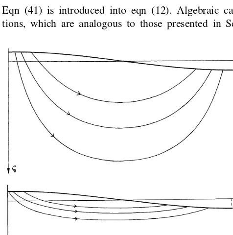
Ifa1q12.1, a streamline which has its starting point in the vicinity of a ‘local ridge’, might have its end point in the vicinity of a ‘local valley’. Even though the starting and end points of a streamline are controlled by the lowest fre-quency, the shape of the streamlines is strongly influenced by the superimposed term. The shallower the streamline, the greater the influence. This is illustrated in Fig. 5, which shows streamlines that are induced by a composed topo-graphy fora1q12¼1.458 andl¼0 and 10.
Fig. 5(a) shows the streamline in a homogeneous rock (l¼0) that passes through (yr¼0.4,zr¼0.05). The resi-dence time isTˆ ¼7.70. The broken line shows the corre-sponding streamline for the undisturbed topography (a1¼ 0). The corresponding residence time isTˆ¼7.05, i.e., about 9% shorter than the value above.
Fig. 5(b) shows two adjacent streamlines in a non homogeneous rock (l ¼ 10), that pass (yr ¼ 0.4, zr ¼ 0.05) and (yr¼0:4;zr¼0:07). The residence time of the
lowest streamline, i.e., the one that does not reach the surface at a local valley, isTˆ ¼ 16.6. The corresponding residence time for an undisturbed topography, (a1¼0), is
ˆ
T¼10.2, i.e., about 40% shorter than for the real streamline. The local flow cells around the local ridges and valleys are well known from the investigation by Toth.13
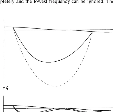
If a1q1 2
q 1, the superimposed term dominates
com-pletely and the lowest frequency can be ignored. Then the
question can arise whether a third superimposed term is important.
2.1.3 Non-periodic topography
If the boundary value fˆs(y) is not periodic, but satisfies
ˆ
f(lyl→`)¼0, the system (12) can be solved by means of Fourier transformation. The transformation:
˜
applied to eqn (12) yields:
d2f˜
The solution of eqn (49) is:
ˆ
The integral in this solution can be evaluated if fˆs(y) is some simple symmetrical (or antisymmetric) function. For these, closed formulae, which correspond to eqn (31)–(40), can be derived. They are somewhat more complicated how-ever.
A simple illustration is a symmetric monotonic boundary value, such as
ˆ
fs(y)¼e¹y2 (52)
Then the Fourier cosine transform applies, which yields:
˜
fs(m)¼ 1
2 p e
¹m2=4 (53)
The character of the flow pattern is sketched in Fig. 6.
The two extremes l p 1 and l q 1 are simple
and illustrative. The calculations below include some
Fig. 6.Streamlines from a single ridge in a space of homogeneous conductivity.
Fig. 5.Streamlines in a semi-space, that are induced by a simple periodic topography with superimposed ridges and valleys. The broken line corresponds to exclusively simple periodic topo-graphy. (a) l ¼ 0 (homogeneous conductivity), (b) l ¼ 10
complicated integrals that can be found in standard tables, e.g., by Gradshteyn and Ryzhik.7
1.lp1.
l → 0 implies thatg ¼ ¹ m, which corresponds to
homogeneous conductivity. Algebraic calculations yield:
ˆ
f(y,z)¼pRe{e¹(yþiz)2erfc(z¹iy)} (54)
The steepest slope offˆs(y) is fory¼1=p2 < 0.707.
This point is a critical point in the sense that a stream-line can only start at the free surface inside this point. At a point at the free surface outside the critical point, water flows out of the domain. The solution, eqn (54), and the corresponding cylindrical solution, have been studied by Rehbinder.9,10
2.lp1
l→`implies thatg¼ ¹1/l. This is not true ifm.
l, but for these m-values, the integrand in eqn (48) is dominated by e¹m2, which is negligible. Algebraic calculations yield the equation of a streamline:
z¼ 1
2lln y y0
(55)
A streamline starting at free surface inside the critical point can never reach the free surface again, which implies that the residence time is infinite.
The first of the extremes is not realistic, but the second is because the horizontal length scale is more likely to far exceed the vertical one. The consequence is that the residence time of a fluid particle is long and that its point of return to the free surface is far from the ridge.
2.2 Frequency spectrum of the elevation of the topography
Possible periodicity of the topography can be identified using either of two methods, which are described below. The basis for all calculations are elevation data in GIS. As mentioned in the introduction, the elevation is given at the nodes of a quadratic mesh. The distance between the points is 500 m. The fact that the mesh is quadratic considerably simplifies the calculations. Details of the topics of this section can be found in the textbook on
multidimen-sional signal processing by Dudgeon and Merserau.5
All numerical calculations which are described below have been performed with the aid of the standard code MATLAB.
2.2.1 Fast Fourier transform
The most straightforward and commonly used frequency analysis is the fast Fourier transform, in the sequel called FFT.
Since the elevationy(k1,k2) is a function of two variables,
the 2D discrete Fourier transform:
Y(n1,n2)¼
applies. An estimate of the power spectrum is then:
ˆ
F(n1,n2)¼lY(n1,n2)l 2
(57)
The amplitude corresponding to a particular frequency is estimated from the FFT as
a¼2lY(n1,n2)l N1N2
(58)
Details on the derivation can be found in the textbook by Brigham.1
Each Fourier coefficient corresponds to the continuous frequencies in each of the two coordinate directions.
q1¼2pn1=N1P1 (59)
q2¼2pn2=N2P2
whereP1andP2are the spatial sampling intervals. Eqn (8) yields the corresponding wavelengths.
L1¼N1P1=n1 (60)
L2¼N2P2=n2
The FFT gives a spectrum defined only by discrete frequency points.
If any of ni is small, i.e., Li,NiPi, the resolution is poor. However, the resolution can be enhanced by the aid of so-called zero-padding. This method is described in the textbook by Brigham.1
2.2.2 Autoregression
Another common method, albeit somewhat more compli-cated, isautoregressioncalled AR in the sequel. In contrast to the FFT, the AR gives the spectrum at any point. On the other hand, the AR does not give any information about the
amplitudeof the components.
According to the AR method, the elevation y(n1,y2) is of which are equal to zero and m respectively. The two-dimensional z-transform applied to eqn (61) yields:
The summation, i.e., the region of supportSmn, remains to be chosen. Here a non-symmetrical half-plane has been used. Hence,
Smn¼{k1,k2lk1¼0, 1#k2#m, 1#k1#n,
¹m#k2#m} ð64Þ
where (m,n) is known as the model order. Estimates of m
and ak1,k2 can be obtained by applying the least squares
method to the elevation data. An estimate of the spectrum in this case is:
ˆ
F(q1,q2)¼ ˆ m
lAˆ(eiq1,eiq2)l2
(65)
Just for the FFT, the dominating length scales are:
L1¼2pP1=q1 (66)
L2¼2pP2=q2
Details on two-dimensional AR-modelling have been reported by Isaksson.8
3 DISCUSSION
3.1 Periodicity of the Swedish topography
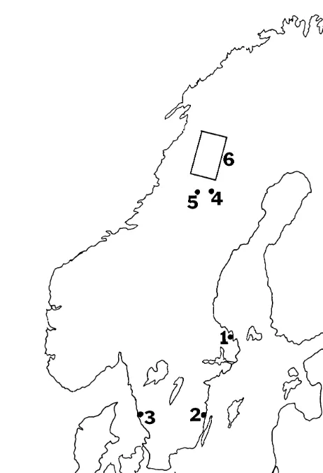
A number of areas in Sweden have been suggested for a future repository of radioactive waste. They are shown in Fig. 7. Forsmark, item 1, and Oskarshamn, item 2, lay at the coast of the Baltic and Ringhals, item 3, at the coast of the Skagerrak. Nuclear power plants are already located at these places. Mala˚, item 5, and Storuman, item 4 in the north, have also been suggested. Most parts of the south of Sweden are low-lying and flat and any possible periodicity of the topography has not been studied. The highland of Sma˚land, between Oskarshamn and Ringhals, is interesting from this point of view. The highland slopes radially and there are good reasons to believe that it has anazimuthal
periodic structure. Such a periodicity, if it exists, cannot be identified because the elevation points are given in a rectan-gular coordinate system. Nonetheless, it does not seem too difficult to investigate azimuthal periodicity, if the GIS points are transformed to polar coordinates.
The dominating hydraulic gradients at Oskarshamn and Ringhals are determined by the ratio between the altitude of the highland of Sma˚land and half the distance between the coasts of the Skagerrak and the Baltic. Analogously, the hydraulic gradient at Forsmark is determined by the ratio between the altitude of southern Norway and the distance between the Caledonian and the Baltic.
In the north, viz., the west part of Lapland, the topography is hilly. Although the Caledonian dominates the topography, there are large valleys with rivers running eastwards to the Baltic. The direction of the rivers is approximately 1208.
The elevation data of some areas in Lapland were analyzed by means of FFT and AR and one specific area, item 6, in Fig. 7, was studied thoroughly. The domain is rectangular,
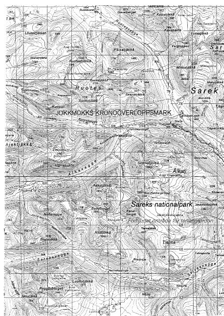
0 # k1# N1, 0# k2# N2. Since the dominating length scale of the Caledonian far exceeds the extent of the domain, the elevation points y(k1,k2) were replaced by reduced points yr(k1,k2), which are equal to the elevation points minus the elevation of the average slope plane of the domain. In this way the dominating period that is equal to infinity is removed. A superficial visual inspection of a standard map, such as the one in Fig. 8, or a level map of the reduced elevation, as the one in Fig. 9, does not give any clear indication whetherperiodicvariations exist within the domain. A preliminary analysis showed that the elevation data can be down-sampled by a factor of 10, without any loss of information. The mesh width of the grid is thus increased to 5000 m. The result of the FFT and AR analyses ofyr(k1,k2) are shown in Figs 10 and 11, respectively.
The fastest frequency that can be represented is given by the Nyquist frequency, which is half the sampling fre-quency, here corresponding to a period of 10 km. The 2-D FFT applied to the domain for whichN1¼40 andN2¼30,
together with zero-padding to 1024 3 1024, yields the
power spectrum which is shown in Fig. 10. It is important to note thatn1andn2in Fig. 10 are running from¹512 to 512. This implies thatN1¼N2¼1024 in eqn (60), whereas
N1¼40 andN2¼30 in eqn (58).
correspond to three sets of periodic topographical waves, viz., (L1¼ 74.2 km,L2 ¼170.7 km, a ¼ 58.2 m), (L1 ¼
146.3 km, L2 ¼ 232.7 km, a ¼ 47.4 m) and (L1 ¼
¹255.7 km, L2 ¼ 204.9 km, a ¼ 46.6 m). The last one
corresponds to the longest wave, whereas the first one cor-responds to the most pronounced wave in the spectrum. Alternatively, every wave can be described as one length scale L¼L1sinvin the direction v¼ arctanL2/L1to the latitude. Hence the shortest, the intermediate and the longest waves, with indicess,iandl, respectively, are (Ls¼68 km,
vs¼678,as¼60 m),Li¼124 km,vi¼588,ai¼47 m) and (Ll¼160 km, vl¼ ¹398,al¼ 47 m). The longest of the above topographical waves can be questioned, since their lengths are approximately the same as or even exceed the extent of the domain.
The AR power spectrum, obtained by estimating a half plane of model order (7,4), is shown in Fig. 11. The peaks are for (q1,q2) ¼(0.49, 0.25), which correspond to L1 ¼ 64 km andL2¼126 km. As above these values correspond toonelength scaleL ¼57 km at an anglev¼638to the
latitude. The longer waves can be discerned, but not evalu-ated. This is in agreement with the comment above, viz., that the number of periods of the long waves in the domain is insufficient.
Despite the reservations, the two methods yield surpris-ingly consistent results, in that the magnitudes as well as the directions of the pronounced topographic waves agree.
Although the shortest wave is dominant in comparison
with the others in Fig. 10, the question is if it is dominant
from a hydraulic point of view, i.e., is the condition
(eqn (47)) sufficiently well violated? The answer is yes, and the reason is the following. Because (as/al)(Ll/Ls)
2
¼
7.1 . 1 and (as/ai)(Li/Ls) 2
¼ 4.3 . 1, it follows that
the influence on the hydraulic gradient of the shortest wave is most likely strong. The lateral length scales are so large, i.e., Ll/z0. Li/z0. Ls/z0q 1 and the location of a possible repository is so shallow, i.e., zr < z0, that the streamlines are very shallow. Consequently, the short but pronounced wave in Figs 10 and 11 determines the flow pattern and the residence time.
3.2 The residence time of a fluid particle
The arguments in Section 3.1 show that in the investigated area, item 6 in Fig. 7, the hydraulic gradient and the stream-lines are determined by two topographical components, one non-periodic and one periodic.
Fig. 9.A contour map of the reduced elevation of the analyzed rectangular area in Fig. 7.
The non periodic length scale that dominates the Scan-dinavian peninsula is half the distance between the Atlantic and the Baltic, i.e.,L,450 km. Large periodic length scale
in the northwest part of Lapland, identified in the previous section, isL,60 km. Both these horizontal length scales far
exceed the vertical length scale that describes the vertical decrease of the conductivity of the bedrock. Consequently the flow of groundwater driven by the variation of the topo-graphy, is confined to a narrow region near the surface, viz.,
zp L.
The flow pattern of the ground water movement is deter-mined by a single dimensionless parameter,
l¼L=2pz0, (67)
if there are periodic ridges, and
z1¹1¼L=2pz1 (68)
if there is a solitary ridge.
The residence time is determined byfourdimensionless
parameters, viz.,
T¼ L
2
4p2f0K0 ˆ
T L
2pz0 ,2pxr
L ,
2pzr L
(69)
A geohydrologist, working practically, would use the peri-odic solution for l q 1, since the results are given as closed formulae. Besides, the estimate of the residential time is conservative. However, a clear periodicity of the topography must exist and be known.
The analysis in Section 2.1.2 can also be used, particu-larly if the topography is known, but its periodicity is unknown or not well established.
If the conductivity is not simple, in the sense that it deviates from eqn (1) or (2), or if the geometry is not simple, the solution of the boundary value problem given by eqn (4)–(9) must be performed with the aid of some numerical method, for example the Finite Element Method. Such an analysis, albeit powerful, requires a detailed knowledge of the complicated conductivity and the complicated geometry. If this knowledge is poor or even non-existant, a simple analysis of the kind mentioned above is preferable.
The magnitude of the residence time is the most important parameter, and if the topography is periodic the simple formulae of eqn (30), (35) and (39) are useful. The following is typical data from the northwestern part of Sweden,
f0.60 m (70)
L.68,000 m,
and the conductivity measurements by Carlsson and Ols-son,2
K0.10¹6m=s (71)
z0.500 m
z1.500 m
indicate thatl.21q1. This means that the streamlines are concentrated to the relative vicinity of the ground surface.
The reference time:
tref¼ L2
4p2f 0K0
.331010s<1000 years (72)
in combination with eqn (39) and (40) yields the shortest residence time
T¼trefTˆ(yr¼p).1:723331010s<1700 years:
(73)
If the repository is located halfway between a ridge and a valley,
T¼trefTˆ(yr¼p=2).3:253331010s<3200 years:
(74)
The above figures must be used with caution, or even sus-picion. The relative error of the residence time is easily Fig. 11.The normalized 2-D power spectrum ofyrdetermined by
derived by logarithmic differentiation of eqn (69). Hence,
and then normalization makes
ˆ either of them, they are negligible compared to dK/K ¼
100–1000. In other words, geometric input data do not need to be refined. One factor that can reduce the residence time is the relation between pore velocity and ‘bulk’ velocity. If K refers to the bulk velocity, the residence time is reduced by a factor that is equal to the porosity. Since the porosity of the bedrock is less than 1%, the resi-dence time might be 1% of the values in eqn (72)–(75). The uncertainty about these things does not affect the analysis. However, the above conductivity refers to the pore velocity.
The above calculation of the flow of groundwater rests upon a number of assumptions. Some of them are physical and others are geometrical. It is clear that all assumptions are not equally uncertain. They are discussed below.
Firstly, the continuum approximation is supposed to be true. This assumption can be questioned, particularly if the residence time is the relevant quantity. If the average flow is the relevant quantity, the large length scale makes the approximation quite acceptable. Secondly, the variation of the topography is assumed to represent the phreatic surface. As mentioned in the introduction, this assumption is most likely valid if the length scale is large.
If the topography contains more than one characteristic wave length, the phreatic surface might do the same. If the phreatic surface contains two such waves, the simple ana-lysis must be extended. Practical experience shows however that the variation of the shape of the phreatic surface is much less than the corresponding ones of the topography.
Thirdly, the existence of possible one-dimensional periodic variations of the topography can rather easily be identified with the aid of FFT or AR of elevation data in GIS. The analysis reveals whether periodicity exists or not, and the wave length and the directions of the waves. Further, the non-homogeneous conductivity can be represented in two similar ways. The fact that the conductivity decreases with depth implies that it can be represented either by the logarithmic formula in an unbounded domain, or by a
homogeneous conductivity in a vertically confined domain. The difference between them is marginal. If the topography is periodic, the former approach is more convenient, because all the results are obtained as simple closed formu-lae. The conductivity data that are collected from scattered spots mainly in the southern part of the country, are sup-posed to be relevant some thousand kilometres further north, which is questionable. The general uncertainty of the conductivity is its enormous spread, making it quite dominant, as pointed out above. Nevertheless, the uncer-tainty is not serious, since the residence time is a linear function of the conductivity. Hence, a calculated residence time can be easily corrected if extended measurements improve the quality of the conductivity data. Finally, a dominant periodicity of the topography must exist and be possible to identify. This last assumption is reasonable pro-vided that the data base in GIS is sufficiently comprehen-sive. In the present case this is true.
4 CONCLUSIONS
The investigation has lead to general and specific con-clusions. It is concluded that in general:
1. The analysis of the large scale flow pattern of ground-water flow in bedrock is particularly simple if the phreatic surface is periodic. The equation of an arbi-trary streamline, an arbiarbi-trary equipotential line and the residence time are simple closed formulae, apt for practical use. If the phreatic surface is character-ized by two or several wave lengths, the longest wave determines the residence time of a fluid particle, if there are no ‘local ridges and valleys’. If there are small ‘local ridges and valleys’ they might or might not determine the residence time. If there are big local ridges and valleys, they determine the flow pattern and the residence time.
2. A possible one-dimensional large-scale periodicity of the phreatic surface, which is identical with the per-iodicity of the topography, can be identified from the
elevation database in Geographic Information
System, with the aid of either fast Fourier transform or autoregression. The resolution of the autoregres-sion is better than that of the fast Fourier transform. 3. The flow pattern is characterized by one geometric
similarity parameter, viz., the ratio between the hori-zontal length scale of the topography and the length scale of the vertical decrease of the conductivity. The residence time of a fluid particle is characterized by
four similarity parameters. Three of them are geo-metric and one is dynamic. The latter, which includes the conductivity, dominates. The residence time increases exponentially with depth of the repository. 4. The relative accuracy of the residence time, which
accuracy of the conductivity. The analysis applied to the situation in Sweden has yielded the following specific conclusions:
5. The horizontal length scale that dominates the Scandinavian peninsula, is characterized by the Caledonian mountain chain. Periodicity occurs in the hilly northwest part of the province of Lapland in northern Sweden. The length scale of the period is approximately 60 km. As a contrast, no periodicity can be identified for the highland of Smland in south-ern Sweden. The latter conclusion can be wrong if the topography of Smland is cylindrically symmetric and contains azimuthal periodicity.
6. The topography of the northwest part of Lapland in combination with the average conductivity of ordin-ary precambrian Swedish rock and the suggested repository depth yields a residence time that is larger than 3000 years. The relative error of the resi-dence time is determined by the relative error of the conductivity, which may be as large as 102–103.
ACKNOWLEDGEMENTS
This investigation has been supported by the Swedish Nuclear Fuel and Waste Management Company. The map in Fig. 8 is published with the permission of the National Land Survey of Sweden under the License Number 97.0045.
REFERENCES
1. Brigham, E. O.,The Fast Fourier Transform and its Applications. Prentice Hall, Englewood Cliffs, NJ, 1988.
2. Carlsson, A. and Olsson, T., Hydraulic Properties of Swedish Crystal-line rock. Hydraulic conductivity and its relation to depth.Bull. Geol. Inst. Univ. of Uppsala N.S., Vol. 7, Uppsala, 1977.
3. Dagan, G. & Nguyen, A. A comparison of travel time and concen-tration approaches to modeling transport by groundwater. J. Con-taminant Hydrol., 1989,479–91.
4. Domenico, P. A.,Concepts and Models in Groundwater Hydrology. McGraw-Hill, NY, 1972.
5. Dudgeon, D. E. and Merserau, R. M., Multidimensional Digital Signal Processing. Prentice Hall, Englewood Cliffs, NJ, 1984. 6. Goode, J. G., Direct simulation of groundwater age.Water Resour.
Res., 1996,32(2), 289–296.
7. Gradshteyn, I. S. & Ryzhik, I. M.,Table of Integrals, Series and Products. Academic Press, NY, 1980.
8. Isaksson, A. J. Frequency domain accuracy of identified 2-D causal AR-models.IEEE Trans. on Signal Processing, 1994,42(2) 399–408. 9. Rehbinder, G. The drag force on a grain in a permeable medium subjected to a water jet.J. Appl. Math. Phys., 1977,281006–1016. 10. Rehbinder, G., Sediment removal with a siphon at critical flux. J.
Hydraulic Res., 1994,32(6), 845–860.
11. Shapiro, A. M. and Cvetkovic, V. D. Stochastic analysis of solute arrival time in heterogeneous porous media. Water Resour. Res., 1988,24(10), 1711–1718.
12. Stokes, J. and Thunvik, R., Investigations of ground water flow in rock around repositories for nuclear waste. KBS Technical Report, Vol. 47, Stockholm, 1978.
13. Toth, J. A. A theory of groundwater motion in small drainage basins in central Alberta.Can. J. Geophys. Res., 1963,684795–4812.
APPENDIX A THREE-DIMENSIONAL SPATIALLY PERIODIC FLOW
The phreatic surface is a two-dimensional structure, and its shape is
fs(y,h)¼cosycosqh,
whereq is the slenderness ratio of the regular bumps that form the topography. The three-dimensional extension of eqn (12) is:
]2fˆ ]y2þ
]2fˆ ]h2þ
]2fˆ ]z2¹l
]fˆ
]z¼0
¹` ,y, `; ¹` ,h, `; 0#z, `
ˆ
f(y,h,z¼0)¼cosycosqh
ˆ
f(y,h,z¼ →`)¼0,
where f(y,h,z) is the three-dimensional potential. The above boundary value problem is solved in analogy with the two-dimensional problem. Hence, algebraic calcula-tions yield a solution that corresponds to eqn (16) and (17),
ˆ
f(y,h,z)¼ef(l)cosycosqh
f(l)¼1
2 l¹
l2þ4(1þq2)
q
: