LOCAL ALGORITHM FOR MONITORING TOTAL SUSPENDED SEDIMENTS IN
MICRO-WATERSHEDS USIN DRONES AND REMOTE SENSING APPLICATIONS.
CASE STUDY: TEUSACÁ RIVER, LA CALERA, COLOMBIA.
N. A. Sáenz a, D. E. Paez a, C. Arangoa
a
Dept. of Environmental and Civil Engineering, Universidad de Los Andes, Cra 1 Nº 18A- 12, Colombia - (na.saenz2751, dpaez, c.arango954)@uniandes.edu.co
KEY WORDS: Geomatics, Water quality, Total Suspended Sediments, Drones (UAVs), Image processing, Remote Sensing.
ABSTRACT:
An empirical relationship of Total Suspended Sediments (TSS) concentrations and reflectance values obtained with Drones’ aerial photos and processed using remote sensing tools was set up as the main objective of this research. A local mathematic algorithm for the micro-watershed of the Teusacá River at La Calera, Colombia, was developed based on the computing of four component of bands from consumed-grade cameras obtaining from each their corresponding reflectance values from procedures for correcting digital camera imagery and using statistical analysis for study the fit and RMSE of 25 regressions. The assessment was characterized by the comparison of reflectance values and 34 in-situ data measurements concentrations between 1.6 and 33 � − taken from the superficial layer of the river in two campaigns. A large data set of empirical and referenced algorithm from literature were used to evaluate the accuracy and precision of the relationship. For estimation of TSS, a higher accuracy was achieved using the Tassan’s algorithm with the BAND X/ BANDX ratio. The correlation coefficient with = � demonstrate the feasibility of use remote sensed data with consumed-grade cameras as an effective tool for a frequent monitoring and controlling of water quality parameters such as Total Suspended Solids of watersheds, these being the most vulnerable and less compliance with environmental regulati ons.
1. INTRODUCTION
Monitoring of water quality in a source is critical to both human health and the environmental sustainability. Despite this, in Colombia no monitoring campaigns are conducted often, not because its importance is not understood but because its implementation involves a high cost in skilled personnel, equipment, laboratory analysis and complex logistics. In addition, traditional water sampling methods for monitoring are able to be performed only at specific points, therefore cannot determine promptly the contaminant concentration throughout the length of the body of water. In the case of Colombia, monitoring is performed by only 154 sampling points in the network of water quality of the IDEAM (Institute of Hydrology, Meteorology and Environmental Studies), having low extension coverage on this issue in the country (IDEAM, 2010).
In terms of finding a technological tool that allows for frequent and cost-efficient monitoring of water quality on different bodies, research has been conducted to study the relationship of remote sensed spectral radiant energy and contaminants concentrations as an alternative methodology for control and monitoring water quality. With this purpose many investigations has been developed in order to find equations to estimate contaminants concentrations based on reflectance values measured by satellite images, allowing control environmental regulations to observe changes in different timeslots and conditions. Studies such as this have been done in different ecosystems within which studies in rivers and lakes of Minnesota (Patrick L. Brezonik, 2007), the coast of Cochin in India (Sravanthi, 2013), studies of water quality in New York Harbor (Hellweger, Schlosser, Lall, & Weissel, 2004), Lake Chicot in Arkansas and the Rio Grande in Texas (Jerry C. Ritchie, 2003) and Lake Balaton (Gitelson & K.Ya.Kondratyev, 1988) are included. However, when it comes to water bodies of smaller area such as micro-watersheds is more complicated to
perform these analyses with high precision, due to the lack of a satellite image with sufficient resolution for accurate results. The high distance existing between the studied object and the satellite leads to obtaining atmospheric noise and curvature error that can affect the data and arriving at a number of erroneous conclusions (Allan, 2008).
Faced with these limitations, a high number of possibilities in the use of new remote sensing tools have been encountered such as Drones, which allow to obtain aerial photographs closest to the target, with higher resolution and can be controlled by the user as needed. Likewise, they are ideal for studies in small areas such as micro-watersheds, one of the richest ecosystems and most important in the abstraction of drinking water.
The conceptual solution presented in this document, is based on the utility of Drones or unmanned aerial vehicles (UAV) and made-consumer grade digital cameras with the purpose of acquire aerial images with high resolution, in order to have the possibility of study micro-watersheds in a technological methodology to manage water quality. The objective is to find a mathematical relationship between the reflectance values obtained by image processing of aerial photographs and the concentration of Total Suspended Solids (TSS) in The Teusacá River at the municipality of La Calera, Colombia, measured by laboratory analysis.
1.1 Study Area
The study area was the Teusacá River located in the municipality of La Calera, Colombia, where it confluence with the Simayá Creek. At this point the mixing plume of both waters presents a high range of TSS concentrations that favor the study. The Teusacá River, a mountain river, was selected for the evaluation of remote sensing tools for monitoring Total Suspended Solids (TSS) concentrations as a water quality The International Archives of the Photogrammetry, Remote Sensing and Spatial Information Sciences, Volume XL-1/W4, 2015
parameter in streams and water bodies. Its Sub-basin is located in the Department of Cundinamarca and is part of the upper basin of the Bogotá River, partially covering the territory of seven municipalities, which use the water as a source of supply for various uses and receiver discharges of wastewater from residential, industrial and agricultural land uses. The Sub-basin, with a total area of 358.17 and annual average flow of 2,2 �3
, was born at 3560 m.s.n.m. in the heights of The Verjón and Los Tunjos Lagoon flowing south-north direction until reaching The Bogotá River.
The specific point where the study was conducted (4.725931° Latitude, -73.949838° Longitude) is important to be close to a Wastewater Treatment Plant (WWTP), which partially addresses the river and discharges on the same, downstream. The sector was considered ideal for the study to allow direct observation of the colour change caused by the differences of Total Suspended Solids in the mixing length interception.
2. MATERIALS AND METHODS
2.1 In-situ sample collection and image acquisition
Field measurements of in-situ Total Suspended Solids (TSS) and reflectance values were carried out by two sampling campaigns in different climatic characteristics on October 4th
and 11th of 2014. From a field trip and a work planning process, 17 points were determined for each campaign, where water samples were recollected using plastic bottles of two litres (2L) due to the water clarity in some sectors. The laboratory of The University of Los Andes, meeting the standards that ensure the maintenance of the sample and the accuracy of the results, performed the sample analyses. In order to define the sampling point in a visible manner on aerial photographs was used as reference element PVC squares supported by ropes at both ends of the river indicating the place where the collection of water samples would take place.
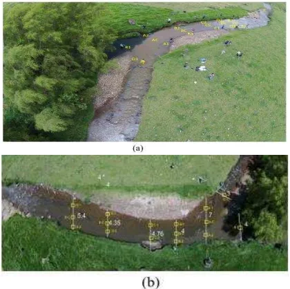
Figure 1 Identification of sample points. (a) Photograph from campaign No. 1. (b) Photograph from the field trip.
The image acquisition was carried out using a Drone Phantom 2 vision+ flying at a height of 30 meters, joined with both a made-consumer digital camera with the traditional bands (RGB or Band 1, 2 and 3) and a Raspberry Pi NoIR Infrared camera (Band 4), as seen in Figure 2.
(a) (b)
Figure 2 (a) Raspberry Pi and NoIR Infrared Camera. (b) Adjustment of the Drone with both cameras.
The camera used to obtain RGB photographs is incorporated into the Drone with Gimbal system that allows stabilizing the camera with 3-axis, uses a CMOS sensor of 14 Mega pixels/180p and allows connection to Wi-Fi network to see the area being covered from mobile devices. Meanwhile, the camera used for Near Infrared (NIR) photographs was a Pi NoIR camera with a resolution of 2592 x 1944 and CMOS sensor of 5 Mega pixels, which works in conjunction with a Raspberry Pi card that was scheduled for take pictures every five seconds (See Figure 2).
Sampling of the first campaign was conducted at the time the WWTP was performing discharges downstream. This time, image sampling was collected with the three main bands, RGB, due to a failure with the NIR camera. On the other hand, the second campaign was conducted during the rainy season presenting high rainfall the previous day, finding a higher flow rate and therefore more dispersed variations in the concentration of TSS. Sampling was done at the time that the WWTP was not discharging and above the same precautions were taken. In this campaign data RGB major bands and Band 4 (NIR) was obtained.
2.2 Image Processing
Use of Drones in the collection of aerial images is a relatively new subject, to find that most such studies have been conducted through the use of satellites and remote sensors. For this type of studies it is necessary to use Reflectance Values, defined as the quantity of energy reflected by a body or surface, because they are characteristics of each object. Conversely, digital units that measure the RGB values can be similar or equal for different objects and its variation range is quite large with aspects such as the incident light intensity. In their regard, the use of digital cameras and Drones must be accompanied by studying of reflectance conversion methods that allows the use of consumer-grade digital cameras to obtain reflectance values from RGB data, to be used for imaging processing.
Although there are many papers on this topic, in this study the image processing was performed in ArcMap using the methodology of (Clemens, 2012), which is used in the AggieAir Flying Circus (AAFC), a service centre at the Utah Water Research Laboratory at the Utah State University, who specializes in the processing and interpretation of aerial images acquired by a UAV system called AggieAir and a consumer-grade digital camera. The methodology used consists of the following steps:
1. Take an after-flight white panel photo captured with both cameras used in the flight mission. The white panel is an object of known and stable reflectance coefficients, and therefore can be used as a reference value to derive correction functions in order to remove the irradiance variations and normalize RGB values of pictures taken with the same camera. The The International Archives of the Photogrammetry, Remote Sensing and Spatial Information Sciences, Volume XL-1/W4, 2015
white panel used in this study was the Barium Sulphate, which is used as a contrast reactive in radiographies.
The realization of the correction and obtaining reflectance values from RGB and NIR acquired with a digital camera is performed for each band separately, so the first thing that was done was the breakdown of the photographs in bands using ArcMap functions. From image processing tools RGB photographs were obtained separated in Band 1, Band 2 and Band 3, i.e. the Red, Green and Blue Bands respectively, In the NIR pictures, being a digital camera, also results in three bands in the Red, Green and Blue spectrum. However, the red band is the closest to the NIR, so this was used in this case.
2. Calculate the Corrected Brightness Value – CBV for each spectral band of the reflectance panel photos. The CBV is a scalar image that allows correct other images taken with the same camera, in order to reduce the irradiance and errors that this effect produces. The CBV is the result of the Correction Coefficient (CC) multiplied by the Brightness Value (BV) of each pixel divided by the transmittance factor �/� , which is the percentage of light passing through the lens of the cameras used. The mathematical representation to calculate the CBV is showed in equation (1), which should be performed for each of the bands used.
� , �, = , �, ∗ ��/�, �,
(1)
The Correction Coefficient (CC) is determined for each band of the white panel photos from the relationship between the Normalized Brightness Value (NBV) and the Brightness Value (BV) of each pixel of the picture in a particular band. The equation is:
, �, , = � ��, �, ,�, , (2)
Where x,y indicate a specific pixel of a particular band, a is the aperture, C is the camera and f is the neutral density filter from which the images were acquired.
The transmittance factor depends on the transmission rate allowed by the filter used, calculated numerically as:
� � =⁄ − (3)
Where d is the percentage of transmittance of the neutral density filter used in the camera lens, it means if the filter allows passing 30% of the light through the lens, d will be equals to 0.3. In oir case any filter was not used, therefore d = 1.
The NBV is calculated for each of the bands as the average of the values of the pixels of withe panel images.
In the case of NIR images equation (2) applies the same way, given that will be used only one Band (Band 1 of NIR images). However, Equation (1) has a
slight shift to note that these cameras does not require the use of filters, therefore the CBV is then:
� , �, = , �, � �, �, (4)
Performing this procedure on each of the bands results in the normalization of values, this process is shown in the standardization of the histogram of the corrected band.
3. Calculate the Reflectance factor – RF for each spectral band for the reflectance panel.
The reflectance factor of the white panel (Barium Sulfate) is determined for each band, which allows relating the RGB values obtained (Digital Units) and reflectance values, thus being a conversion factor. The reflectance factor �� depends on known reflectance coefficients, A , A , A , A y A , and the zenith angle θz:
��= + ∗ �� + ∗ �� + ∗
�� + + �� (5)
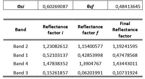
The reflectance coefficients were found in (Clemens, 2012). Reflectance factors for the start time and end time of the flight, with the zenith angle of flying day and specific coordinates were calculated. Table 1 shows the results for 10:00 a.m. and 10:15 a.m. showing as final reflectance value of the average of the two to find a short-duration flight.
Table 1. Reflectance factor results
Θzi 0,60269087 θzf 0,48413645
Band Reflectance
factor i
Reflectance factor f
Final Reflectance
factor
Band 2 1,23082612 1,15400577 1,19241595
Band 1 0,52103137 0,42853998 0,47478568
Band 4 1,47838352 1,3904767 1,43443011
Band 3 0,15261857 0,06201991 0,10731924
4. Calculate the reflectance image for individual bands. The reflectance image is the final result of the conversion of digital number to reflectance values, which depends on the reflectance factor, the original image and the CBV of the white panel in the particular band. This process has to be performed for each of the bands. The mathematical representation is:
� �� � , =
� �� �� � � �, , � � � , �, ,
� � � �, , (6)
The outputs of the RGB reflectance model were individual layers of each band expressed as reflectance values.
5. Get the reflectance values necessary for the statistics analysis.
The determination of the reflectance value for each sample point was developed with the ArcMap tool Image Classification, which allows realizing a polygon in order to delimit the area of sampling and obtain their mean reflectance value. This process was executed for each sampling point for the four bands, determining the mean reflectance value for each one.
The result was a table that relates reflectance values and TSS concentrations of 34 sampling point, 17 for each campaign. The relationship found between TSS concentrations and the four bands was the expected, founding that the higher concentration levels increase reflectance of the water body have greater ability to reflect light, while at lower concentration will decrease.
2.3 Statistical correlation analysis and regression models
The methodology followed for the statistical analysis and regression models includes:
1. Analysis of covariance between TSS concentration and each of the bands using Matlab.
The analysis of covariance provides information about the relationship between the independent and dependent variables. This analysis was performed using the functions provided by Matlab, with which it results the covariance matrix for each of the variables analysed:
Table 2 Covariance matrixes for each band
TSS B1 TSS B2 determination of TSS. For its part, the variables Band 4, Band 1 and Band 2 have a direct relationship with a level of significance in that order. However, the correlation with bands 1 and 2 is more relevant due to the greater amount of data used regarding the analysis of band 4.
2. Completing the ascendant method for performing regressions to find the best fit.
The ascendant method is a process for performing multiple regressions considering mainly the level of significance of each independent variable with respect to the determination of the dependent variable. The procedure involves initial conducting with each independent variable separately in order to determine the level of significance through the P-Value and adding to the regression more variables to complete multiple regressions. Using this process 25 regression models were performed with Matlab and the Excel
tool data analysis for being analysed with goodness fit.
In order to obtain evaluation tools for the mathematical adjustments five values of the sampled data were excluded of the regressions, and then calculate their TSS concentrations with the equations and compare with the actual values.
3. Determination of statistics for each regression and analysis of variance to determine the significance of each parameter and analysis of goodness of fit.
Statistical variables which were used for analysis of goodness of fit were primarily the coefficient of determination ( ), the adjusted coefficient of determination (Adj. ), the Root Mean Square Error (RMSE), analysis of variance with F-Fisher, analysis of the plot residuals and significance levels from P-Value with 95% of reliability.
4. Use each regression to determine TSS concentrations of excluded values and calculate RMSE of this data.
Regressions validation was performed from the comparison of each of the statistical parameters analysed, moreover were calculated TSS concentrations of excluded values and compared with the actual data from RMSE. This statistical parameter allows define the validity of the adjustment for values obtained in the sampling process, the lower was the RMSE for the regression would have greater weight to be selected.
5. Analyse the obtained statistical parameters and determine the regression that best fits the data. After an analysis of each of the regressions fit models, best fits with better characteristics for the observed data were defined. Likewise, regressions with minor adjustment and variables with less level of significance were also defined.
3. RESULTS AND DISCUSSION
In this study, the analysis of multiple linear regression were performed using combination of variables considering the empirical trends found from the presented covariance and theoretical algorithm from literature. Sravanthi, N. et al. (2013) have observed on coastal waters off Cochin a progressive increase in reflectance in the visible region as suspended sediment concentrations increase. This relationship was observed equally in the measurements of the Teusacá River, determining a relationship between TSS concentrations and Reflectance values in the visible region and near IR band.
The best linear relationship observed in Sravanthi, N. et al.’s
study was presented as [ + ]/ [�
� 9 ] , observed a strong correlation between square of ratio of Band 1 and Band 3 and a weak correlation between the ratio of near IR and Band 2. A.A. Gitelson. et al. (1991) tested the relationship between optical indices and Suspended Mineral Matter for the Don, the Tsymlianskoe reservoir and the Sea of Azov, founded that the most efficient index was [ − ]/ [ + ]. Further studies of S. Tassan in coastal waters (1994) tested the algorithm with the form = [ � + (� )][� �� � ]�where the first factor is the sensitive The International Archives of the Photogrammetry, Remote Sensing and Spatial Information Sciences, Volume XL-1/W4, 2015
term and the second factor is the compensating term resulting in = [ + ] [� 9� ]− . , observed a strong correlation with Band 2 and Band 1 and a lower correlation with the ratio of Band 2 and Band 1.
Asif M. Bhatti et al. presents an algorithm that predicts Suspended Sediments Concentrations in water bodies using the combination � + � / � /� and Total Suspended Sediments using the quadratic algorithm = �
� −
� � + .
This study suggests a strong correlation between TSS measured concentrations and Band 4 (Near IR), Band 2 (Green) and Band 1 (Red), even in algorithms derived with single wavelengths, and a weak correlation with Band 3. However, from results found in literature, the use of a ratio of bands or combination of different wavelengths in a linear regression is closer to reality. Indeed, single algorithms were tested in order to validate the correlation between TSS and reflectance values, further empirical and theoretical algorithms were tested analysing the best adjustment.
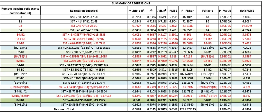
Table 4 presents the coefficient of determination and Root Mean Square Error (RMSR) of different regressions for various combinations of the wavelength bands, showing in green and blue regressions with high goodness of fit values, however there is a distinction between then, where the blue colour represents the quadratic regression and green colour linear regressions.
Although best values of adjusted coefficient ( of determination were found to quadratic regressions than for linear regressions, the choice of the algorithm was based on the RMSE of the excluded values. Given this, regression chosen to define the relationship between the concentration of TSS and reflectance values is:
(7)
Finding an adjusted of 0.8781, RMSE of 3.4827, the validation of the hypothesis test for F-Fisher and lower RMSE from excluded values.
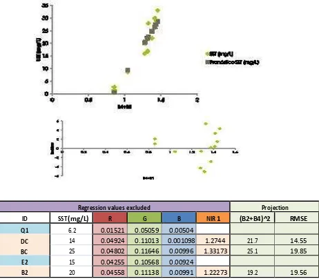
Regression values excluded Projection
ID SST (mg/L) R G B NIR 1 (B2+B4)^2 RMSE
Q1 6.2 0.01521 0.05059 0.00504
DC BC
14 0.04924 0.11013 0.001098 1.2744 21.7 14.55 25 0.04802 0.11646 0.00996 1.33173 25.1 19.85
E2 15 0.04255 0.10568 0.00924
B2 20 0.04558 0.11138 0.00991 1.22273 19.2 19.56
Figure 3 RMSE for excluded values, linear regression fit between in situ TSS and reflectance values and residual curve.
The linear regression fit between in situ TSS and reflectance values and residual curve show a good relationship between the sum of Band 4 and Band 1, presenting a chart scattered and good estimated values.
In addition, algorithms from literature were tested calculating their coefficient of determination and Root Mean Square Error for the data measured in the Teusacá River. It is found better goodness of fit from these statistical determinants, noticing that this references use the most sensitive bands found in the results of this study. Tassan’s algorithm presents a high coefficient of determination and a good RMSE combining the bands 2 and 4 as the sensitive term and a ratio of bands 1 and 2 for the compensating term. Algorithm used by Asif M. Bhatti et al. for estimate Suspended Sediments Concentrations in water bodies presents a high goodness of fit, while the algorithm for Total Suspended Sediments has low coefficient of determination. Algorithm from Sravanthi, N. et al. presents a good coefficient of determination but a high RMSE, while Gitelson. et al. algorithm presents a low goodness of fit for both determinants.
Table 3 Algorithm from literature evaluated for Teusacá River measurements.
Equation 7 was compared with Tassan’s algorithm through the use of these in Arcmap to observe the distribution of TSS estimated by each. It was found that although Tassan’s algorithm has better statistical fit, does not represent the behaviour of the river according to the measurements made in the campaigns. On the other hand, Equation 7 represents a distribution according to measurements, but it is observed an overestimation and low accuracy in the pixels of the edges, characteristic problem of satellite and digital images. For this reason, although Equation 7 requires an important validation process is chosen over other algorithms evaluated.
Figure 4 Comparing distributions estimated by Tassan’s
algorithm and Equation 7
SUMMARY OF REGRESSIONS Remote sensing reflectance
combination (X) Regression equation Multiple R² R² Adj. R² RMSE F - Fisher Variable P - Value data RMSE
B1 SST = 900.6*B1-17.58 0.7953 0.6326 0.619 5.252 46.4821 B1 2.53E-07 7.8745
B2 SST = 414.5*B2-22.43 0.8543 0.7298 0.7198 4.504 72.9307 B2 3.74E-09 6.3084
B3 SST = 4870*B3-23.06 0.7427 0.5516 0.535 5.802 33.2116 B3 3.96E-06 14.8549
B4 SST = 48.47*B4-39.594 0.9431 0.8894 0.8802 3.451 96.5531 B4 4.33E-07 4.7244
B4/B2 SST = -8.47597*(B4/B2)+119.5333 0.6031 0.3637 0.3107 8.2801 6.861 B4/B2 2.24E-02 5.8673
B3 + B2 SST = 386.2681*(B3+B2) -22.96 0.8508 0.7238 0.7135 4.5536 70.7592 B3+B2 5.05E-09 5.5162
B2-B3 SST = 446.4573*(B2-B3) - 21.7411 0.8576 0.7354 0.7256 4.4566 75.0628 B2-B3 2.80E-09 7.4621
(B2-B3)^2 SST = 2710.61193*(B2-B3)^2 -4.51366235 0.8681 0.7535 0.7444 4.3017 82.5467 (B2-B3)^2 1.07E-09 7.2023 B2-B1 SST = 681.58*(B2-B1)-21.23 0.8492 0.7212 0.7109 4.5747 69.8606 B2-B1 5.73E-09 4.6862
(B4/B2)^2 SST = -0.35546*(B4/B2)^2+69.18095 0.5989 0.3587 0.3052 8.313 6.7119 (B4/B2)^2 2.36E-02 5.8597
B2+B1 SST = 289.703*(B2+B1)-21.7618 0.8447 0.7135 0.7029 4.6376 67.2520 B2+B1 8.32E-09 6.9323
B4-B1 SST = 50.4758471*(B4-B1)-39.9071347 0.9442 0.8915 0.8824 3.4197 98.5784 B4-B1 3.87E-07 4.5898
B4-B2 SST = 53.60182*(B4-B2)-40.2524 0.9386 0.8809 0.871 3.5815 88.8105 B4-B2 6.77E-07 4.7249 (B4-B2)^2 SST = 26.70806*(B4-B2)^2-14.477 0.9485 0.8997 0.8914 3.2871 107.6781931 (B4-B2)^2 2.40E-07 4.5431
B2+B4 SST= 44.17004*(B2+B4)-38.9587 0.9461 0.8951 0.8863 3.3628 102.3481 B2+B4 3.16E-07 4.732
(B2+B4)^2 SST=18.5244*(B2+B4)^2-13.7644 0.9563 0.9145 0.9073 3.0361 128.2875 (B2+B4)^2 9.18E-08 4.4955
(B2+B4)^2/(B2) SST = 3.54985*((B2+B4)^2/B2)-40.2167 0.8567 0.7339 0.7117 5.355 33.0936 (B2+B4)^2/(B2) 9.12E-05 4.871
(B4-B1)^2 SST = 23.77366*(B4-B1)^2 - 14.2304 0.9541 0.9103 0.9028 3.1089 121.7912 (B4-B1)^2 1.22E-07 4.3676
B2+B1/ B2+B4 SST = 1245.508*(B2+B1)/(B2+B4) - 117.612 0.6346 0.4027 0.3529 8.0224 8.0921 B2+B1/ B2+B4 1.48E-02 8.547
B4+B1 SST = 46.61479*(B4+B1)-39.2955 0.942 0.8874 0.8781 3.4827 94.6101 B4+B1 4.83E-07 4.2414
(B4+B1)^2 SST = 20.56439*(B4+B1)^2 -14.0236 0.9525 0.9074 0.8996 3.1593 117.5560 (B4+B1)^2 1.48E-07 4.6546
Resumen Total 0.9563 0.9145 0.9073 3.0361128.2875125 1.07E-09 4.2414
Figure 5 Summary of regressions. Coefficient of determination ( ) and Root Mean Square Error (RMSR) of different regressions for combinations of the wavelength bands. Colour red for low goodness of fit regressions, blue for quadratic
regressions with high goodness of fit and green for linear regressions with high goodness of fit.
Having obliquity in the photograph was not possible to observe an orthophoto that would allow entire length of the river studied, therefore there is shown two photographs separately. A reclassification in 30 categories was performed in order to observe carefully changes in concentrations of TSS. The distribution found is consistent with the expected results, finding that the chosen regression is a good fit and can effectively relate TSS concentrations with Reflectance values obtained from aerial images.
3.1 Advantages and limitations
Satellites are tools that have been very useful in studies concerning remote sensing helping the understanding of water quality in streams and water bodies of great extent. However, it has several limitations that the use of Drones can supply, such as the lack of precision for smaller water bodies, lack of control of the tool according to the user requirements, problems of high cloud cover and curvature errors, control altitude sensor, among others.
Although Drones have great advantages, they also have limitations in terms of weather conditions with low wind speed and rainfall. Additionally, it is necessary to choose Drone features regarding the extent of the area to cover, which may have higher costs.
Related to the methodology used, it is the opportunity to have a tool of control and monitoring of water quality. In this case to determine the Total Suspended Solids, which allows spatiotemporal analysis and reaches greater compliance environmental regulations on the subject. The efficiency of the methodology allows knowing the concentration of the water quality determinant in the entire length of the river with only obtaining aerial photographs of the area using consumer-grade cameras.
The relationships found with high levels of goodness of fit for the tested regressions confirms the effectiveness of the proposed methodology and the speed and effectiveness where it is possible to determine the concentration of TSS and its display on a map of their distribution.
The validation process should be performed both in the studied river and in other rivers to be used reliably. In addition, reflectance values measurements depend on variables such as the intensity of light source (location, weather conditions and time of the day), camera angularity and characteristics of the river bed.
4. CONCLUSION
The main objective of this study was based on the evaluation of the relationship between the concentration of Total Suspended Solids with reflectance values obtained from aerial images acquired with a Drone. The analysis was performed from the case study Teusacá River located in the municipality of La Calera in Colombia, from two sampling campaigns where quality information and aerial photographs were collected.
From this analysis, an empirical relationship has been established between reflectance values and concentration of Total Suspended Solids observed a high correlation with wavelengths band 4 (Near IR), Band 2 (Green) and Band 1 (red). A correlation with a coefficient of determination of 0.8781 was obtained derived from band combinations of Band4 and Band 1 and in situ measures of TSS.
In addition, a methodology for the transformation of digital numbers to reflectance levels was performed, testing the applicability of aerial photographs taken from Drones and consumer-grade cameras to analyse determinants that affect water quality. From this procedure, a specific methodology for using remote sensing tools such as Drones as control and monitoring of water quality in watersheds was obtained, having a significant positive impact, being these bodies to be more vulnerable and difficult to observe from high distance instruments such as satellites.
The evaluation of the methodology used in this study is a starting point for research into the use of remote sensing in determining water quality, from which other research possibilities and modelling are released. Studies would be defined in other water bodies, steady control of water pollution, enhance and validate the methodology as many sampling points and greater resources and evaluation of relations with other determinants of water quality.
It was found possible to carry out a visual map of the distribution of the concentration of the pollutant in the river from the advantages of the use of Drones. However, accuracy problems were observed on the edges so it is recommended to obtain photographs with little obliquity in order to be able to produce an orthophoto where the sector study is centred in the image.
5. REFERENCES
Allan, M. G. (2008). Remote Sensing of Water Quality in Rotorua and Waikato Lakes. The University of Waikato. The University of Waikato.
Bhatti, A. M., Rundquist, D. C., Nasu, S., & Takagi, M. ASSESSING THE POTENTIAL OF REMOTELY SENSED DATA FOR WATER QUALITY MONITORING OF COASTAL AND INLAND WATERS.
Clemens, S. R. (2012). Procedures for correcting Digital Camera Imagery Acquired by the AggieAir remote sensing platform. Utah: Utah State University.
Gitelson, A., & K.Ya.Kondratyev. (1988). Optical models of
mesotriphic and eutrophic water bodies. Remote sensing , 373-
38 5.
Gitelson, A., & Kondratyev, K. (1991). Optical Models of mesotrophic and eutrophic water bodies. INT. J. REMOTE SENSING.
Hellweger, F., Schlosser, P., Lall, U., & Weissel, J. (2004). Use of satellite imagery for water quality studies in New York Harbor. Estuarine, Coastal and Shelf Science , 437-448.
Honkavaara, E., Hakala, T., Markelin, L., & Peltoniemi, J. (2014). METROLOGY OF IMAGE PROCESSING IN SPECTRAL REFLECTANCE MEASUREMENT BY UAV. Photogrammetry, Remote Sensing and Spatial Information Sciences.
IDEAM. (December de 2010). Sistema de información ambiental de Colombia. Obtenido de Estudio Nacional del agua
201 0:
https://www.siac.gov.co/documentos/DOC_Portal/DOC_Agu a/
3_Estado/20120928_Estado_agua_ENA2010PrCap1y2.p df
Jerry C. Ritchie, P. V. (2003). Remote Sensing Techniques to Assess Water Quality. Photogrammetric Engineering & Remote Sensing , 69, 695–704.
Kali E. Sawaya, L. G. (2002). Extending satellite remote sensing to local scales: land and water resource monitoring using high-resolution imagery. University of Minnesota. Minnesota: ELSEVIER.
Keith, D. J. (2014). Satellite remote sensing of chlorophyll a in support of nutrient management in the Neuse and Tar– Pamlico River (North Carolina) estuaries. Remote Sensing of Environment.
Patrick L. Brezonik, L. G. (2007). Measuring Water Clarity and Quality in Minnesota Lakes and Rivers: A Census-Based Approach Using Remote-Sensing Techniques. University of Minnesota. Minnesota: CURA REPORTER.
R, R., S, M., & A, D. (2013). Environmental monitoring of estuaries: Estimating and mapping various environmental indicators in Matla estuarine complex, using Landsat TM digital data. INTERNATIONAL J OURNAL OF GEOMATICS AND GEOSCIENCES .
R. CHOPRA, V. K., & SHARMA, P. K. (2001). Mapping, monitoring and conservation of Harike wetland ecosystem, Punjab, India, through remote sensing. int. j. remote sensing,
22, 89-98.
Ritchie, J., Zimba, P., & Everitt, J. (2003). Remote sensing techniques to assess water quality. Photogrammetric engineering & remote sensing.
Sravanthi, N., Ramana, I., Ali, P. Y., Ashraf, M., Ali, M., & Narayana, A. (2013). An Algorithm for Estimating Suspended Sediment Concentrations in the Coastal Waters of India using Remotely Sensed Reflectance and its Application to Coastal Environments. INT. J. ENVIRONMENT.
Sravanthi, N. R. (2013). An Algorithm for Estimating Suspended Sediment Concentrations in the Coastal Waters of India using Remotely Sensed Reflectance and its Application to Coastal Environments. Int. J. Environment.
Wang, F., & Xu, Y. J. (2008). Development and application of a remote sensing-based salinity prediction model for a large estuarine lake in the US Gulf of Mexico coast. Journal of Hydrology.
Whitman College. (n.d.). Total Suspended Solids in Water Samples. Retrieved from Whitman College:
http://www.whitman.edu/chemistry/edusolns_software/TSSBa c kground.pdf
Yuanzhi Zhang, J. P. (2002). Application of an empirical neural network to surface water quality estimation in the Gulf of Finland using combined optical data and microwave data. Remote sensing of environment, 327-336