TERRESTRIAL LASER SCANNING FOR PLANT HEIGHT MEASUREMENT AND
BIOMASS ESTIMATION OF MAIZE
N. Tilly a,*, D. Hoffmeister a, H. Schiedung b, C. Hütt a, J. Brands a, G. Bareth a
a Institute of Geography (GIS & Remote Sensing Group), University of Cologne, 50923 Cologne, Germany - (nora.tilly, dirk.hoffmeister, christoph.huett, jbrands1, g.bareth)@uni-koeln.de
b Institute of Crop Science and Resource Conservation, University of Bonn, 53121 Bonn, Germany [email protected]
Commission VII, WG VII/5
KEY WORDS: TLS, Multitemporal, Agriculture, Crop, Change Detection, Monitoring
ABSTRACT:
Over the last decades, the role of remote sensing gained in importance for monitoring applications in precision agriculture. A key factor for assessing the development of crops during the growing period is the actual biomass. As non-destructive methods of directly measuring biomass do not exist, parameters like plant height are considered as estimators. In this contribution, first results of multi-temporal surveys on a maize field with a terrestrial laser scanner are shown. The achieved point clouds are interpolated to generate Crop Surface Models (CSM) that represent the top canopy. These CSMs are used for visualizing the spatial distribution of plant height differences within the field and calculating plant height above ground with a high resolution of 1 cm. In addition, manual measurements of plant height were carried out corresponding to each TLS campaign to verify the results. The high coefficient of determination (R² = 0.93) between both measurement methods shows the applicability of the presented approach. The established regression model between CSM-derived plant height and destructively measured biomass shows a varying performance depending on the considered time frame during the growing period. This study shows that TLS is a suitable and promising method for measuring plant height of maize. Moreover, it shows the potential of plant height as a non-destructive estimator for biomass in the early growing period. However, challenges are the non-linear development of plant height and biomass over the whole growing period.
1. INTRODUCTION
A major topic in the field of precision agriculture (PA) is the enhancement of crop management due to the constant or even decreasing cultivation area but concurrently growing world population (Oliver, 2013). Therefore an accurate determination of the crop status during the growing period is required. In the last decades, remote and proximal sensing methods are widely used for crop monitoring. Depending on the investigated parameters and desired resolution various sensors and methods are applied. An overview is given in Mulla (2013).
Studies focusing on maize plants have a particular challenge in common. In contrast to other crops, tall maize plants with heights of about 3 m complicate ground based nadir measurements. As demonstrated by Claverie et al. (2012), spectral satellite data has promising potential for large-scale crop monitoring and biomass estimation. However, ground based observations are conducted to achieve a high resolution and thus enable the detection of infield variability. Studies show the potential of passive hyperspectral hand-held sensors for biomass estimations (Teal et al., 2006; Osborne et al., 2002). Perbandt et al. (2011) compared nadir and off-nadir hyperspectral measurements and detected a significant influence of sensor height and measuring angle.
A major disadvantage of passive sensors is the dependency on solar radiation. By contrast, studies show that terrestrial laser scanning (TLS), as an active system, can be applied for agricultural purposes. Investigated plant parameters are plant height (Zhang and Grift, 2012), biomass (Keightley and Bawden, 2010; Ehlert et al., 2009; 2008), crop density (Hosoi and Omasa,
* Corresponding author: [email protected]
2012; 2009; Saeys et al., 2009), and leaf area index (Gebbers et al., 2011). As mentioned the large height of maize plants causes difficulties for ground based system. Solely, Höfle (2014) used the measured intensity values from TLS for detecting single plants of maize.
In this contribution, the first results of multi-temporal surveys on a maize field with a TLS system are shown. The scanner was mounted on a cherry picker to reach a high position above the canopy. The TLS-derived point clouds are interpolated to generate Crop Surface Models (CSM) that represent the top canopy. The concept of CSMs for determining plant height and estimating biomass was tested for sugar beet (Hoffmeister et al., 2013; 2010), barley (Tilly et al., 2014a) and paddy rice (Tilly et al., 2014b).
2. METHODS
2.1 Data acquisition
In the growing period 2013, surveys were carried out on a maize field in Selhausen, about 40 km away from Cologne, Germany
(N 50°52’5”, E 6°27’11”). The field with a spatial extent of about 60 m by 160 m was chosen, due to heterogeneous soil conditions and thereby expected differences in plant development within the field. Six field campaigns were carried out between the 22nd of May and 24th of September 2013 for monitoring plant height. Thus, almost the whole growing period of maize is covered. For an accurate acquisition of the ground surface the first campaign was scheduled after sowing, before the plants are visible above ground.
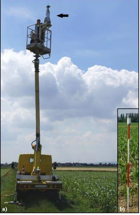
For all campaigns, the terrestrial laser scanner Riegl LMS-Z420i was used, which applies the time-of-flight method (Riegl GmbH, 2010) (Fig. 1a)). From the known position of the scanner, the position of targets is calculated by measuring the distance through the time shift between transmitting and receiving a pulsed signal and the respective direction. The laser beam is generated in the bottom of the device with a measurement rate of up to 11,000 points/sec. Parallel scan lines are achieved with a rotating multi-facet polygon mirror and the rotation of the scanners head. Thereby a wide field of view can be achieved, up to 80° in vertical and 360° in horizontal direction. Furthermore, a digital camera, Nikon D200, was mounted on the laser scanner. From the recorded RGB-images, the point clouds recorded by the scanner can be colorized and the corresponding surfaces can be textured.
The scanner was mounted on a cherry picker to achieve a high position above the canopy (Fig. 1a)). The height of the sensor was about 8 m above ground. All positions of the scanner were measured with the highly accurate RTK-DGPS system Topcon HiPer Pro (Topcon Positioning Systems Inc., 2006). The relative accuracy of this system is ~1 cm. Additional reference targets are required to enable a direct georeferencing in the postprocessing. Therefore, highly reflective cylinders arranged on ranging poles were used, which can be easily detected by the laser scanner and their coordinates were measured with the RTK-DGPS system (Fig. 1b)). In each campaign, the field was scanned from its four corners for achieving a uniform spatial resolution and lower
shadowing effects. For all scans a resolution of 0.7 cm at a distance of 10 m was used.
With exception of the first campaign, manual measurements of plant height and biomass were carried out, corresponding to the TLS measurements. Therefore twelve sample points, well distributed in the field, were marked in the first campaign and their positions were measured with the RTK-DGPS system. Hence, the manual and TLS measurements can be accurately linked. In each campaign, the heights of five plants per sample point were measured. In the last four campaigns, destructive sampling of biomass was performed. Around each sample point, five plants were taken after the TLS and manual height measurements.
2.2 Data processing
The workflow for the postprocessing can be divided in three main steps: (i) the registration and merging of all point clouds; (ii) the extraction of the Area of Interest (AOI), both executed in Riegl's software RiSCAN Pro; (iii) spatial analyses, conducted in ArcGIS Desktop 10 by Esri; and (iv) statistical analyses, calculated with Microsoft Excel 2013 and diagrams plotted in OriginPro 8.5 by OriginLab.
At first, the scan data from all campaigns and the GPS-derived coordinates were imported into one RiSCAN Pro project file. Based on the positions of the scanner and the reflectors, a direct georeferencing method was used for the registration of the scan positions. However, small alignment errors occur between the point clouds of one campaign and between different campaigns. Thus, a further adjustment was applied. RiSCAN Pro offers the Multi Station Adjustment, where the position and orientation of each scan position are modified in multiple iterations to get the best fitting result for all of them. The calculations are based on the Iterative Closest Point (ICP) algorithm (Besl and McKay, 1992).
Following, all point clouds of one date were merged to one data set and the AOI was manually extracted. Moreover, points regarded as noise were removed, caused by reflections on insects or other small particles in the air. The crop surface was then determined from the data sets with a filtering scheme for selecting maximum points. Similar, for the data set of the first campaign a filtering scheme for selecting minimum points was used to extract ground points. Finally, the data sets were exported for the following analyses.
In ArcGIS Desktop 10, the exported point cloud data sets were interpolated with the Inverse Distance Weighting (IDW) algorithm. For retaining the accuracy of measurements with a high density, this exact, deterministic algorithm is well suitable as measured values are retained at their sample location (Johnston et al., 2001). The result are raster data sets with a consistent spatial resolution of 1 cm, introduced by Hoffmeister et al. (2010) as Crop Surface Models (CSMs). For each date, the CSM represents the crop surface of the whole field in a high resolution. Hence, infield variability can be spatially measured. A Digital Elevation Model (DEM) is interpolated from the ground points of the first campaign as a common reference surface for the calculation of plant heights. By subtracting the DEM from a CSM, the actual plant height is calculated with the same spatial resolution. Likewise, by calculating the difference between two CSMs the plant growth can be spatially measured for the respective period of time. Herein, growth is defined as a temporal difference in height.
Fig. 1 a) TLS system (marked with arrow) mounted on a cherry picker; b) highly reflective cylinders arranged on ranging pole.
Furthermore, statistical analyses were performed, taking account of the manual measurements. For validating the TLS results, a common spatial base was required. Therefore, a circular buffer with a radius of 1 m was generated around each sample point, where the CSM-derived plant heights were averaged (n = 12). The manually measured plant heights and destructively taken biomass were also averaged for each sample point. Consequently, correlation and regression analyses were carried out to investigate the accuracy of the TLS results and examining the usability of plant height as predictor for biomass of maize.
3. RESULTS
3.1 Spatial analysis
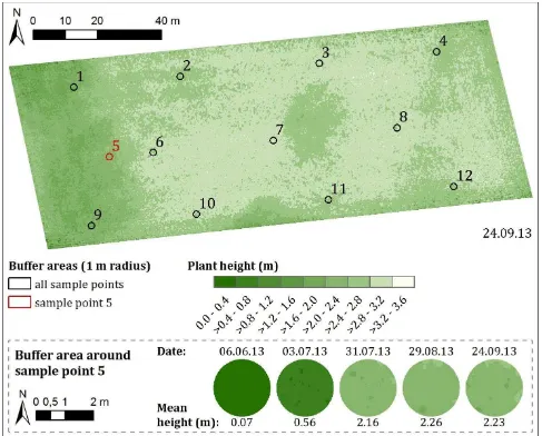
The TLS-derived point clouds were interpolated to generate a CSM of the whole maize field for each campaign. By subtracting the DEM from each CSM, the plant heights are calculated pixel-wise for the whole field and visualized as map of plant height for each campaign. Thus, spatial differences in plant height and their temporal development can be detected. As an example, Figure 2 shows the maps of plant height for the whole field on the last campaign date and for the buffer area around sample point 5 on each date. Regarding the whole field, spatial patterns are observable. It has to be mentioned that the whole field was clipped with an inner buffer of 1 m for avoiding border effects.
However, in particular in the corners such influences cannot be completely excluded and the south edge of the field seems to be more affected. Nevertheless, spatial patterns are noticeable. Lower plant height values are detectable (i) in a stripe of ~20 m at the west edge, (ii) in an almost circular area with a diameter of ~15 m eastward of sample point 7, and (iii) in a small area at the south edge between the sample points 10 and 11. Regarding the detailed view of the buffer area around sample point 5, the plant height increase between the campaigns is clearly detectable for the first half of the observation period. However, as also supported by the mean values, the plant height is almost constant from late July to the end of the observation period in late September.
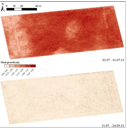
The spatial distribution of plant height differences between the campaigns is measured by subtracting the CSM of an earlier date from the CSM of a later date and visualized in maps of plant growth. In Figure 3, maps of plant growth are shown for two time periods. At the top, the plant growth between the 3rd and 31st of July and at the bottom between the 31st of July and the 24th of September are shown. Thereby the above stated results are supported. On the on the hand, for the earlier period, the same spatial patterns with areas of lower plant growth are detectable at the west edge, in the almost circular area in the middle, and in the small area at the south edge. On the other hand, the temporal
Fig. 2 CSM-derived maps of plant height for the whole maize field on the last campaign date (top) and for the buffer area around sample point 5 on each date (bottom).
development, stated for the buffer area around sample point 5 is also observable. The main increase occurred in July with a mean plant growth of about 2 m for the whole field, whereas afterwards the plant heights are almost constant with a mean growth of 0.08 m for the whole field until the end of September.
3.2 Statistical analysis
Besides the visualization of spatial patterns, the quantification of plant height differences and the correlation between plant height and biomass was an object of this study. The analyses are based on the averaged values, measured in the buffer areas around the sample points. Table 1 gives the mean value ( ), standard deviation (s), minimum (min), and maximum (max) for the CSM-derived and manually measured plant heights, as well as for the destructively taken biomass. Regarding the plant height, the results of both measuring methods are similar. The differences
can be summarized as: (i) except of the first campaign, the CSM-derived values are always a little higher, (ii) the standard deviations are very similar, (iii) in conformity with the mean values, the minimum and maximum values are mainly a bit lower for the CSM-derived values. As already stated for the maps of plant growth, the main increase occurred in July. Afterwards the plant heights are almost constant.
Regarding the biomass, no comparative statements can be done. Nonetheless, it is noteworthy that in contrast to the almost constant plant height in the second half of the observation period, the biomass still increases. However, the main increase occurred in the first half, between the 3rd and 31st of July where the amount increased about 60 times. It has to be mentioned, that the values for the samples of the 31st of July are a little too high. Due to technical problems, some plants were not completely dry while weighing. Consequently the plants were heavier owing to the Fig. 3 CSM-derived maps of plant growth for the whole maize field (At the top between 3rd and 31st of July; at the bottom between the 31st of July and the 24h of September).
remaining water. As the problem could not be fixed and the amount of water could not be determined afterwards, the values were used for the analyses. Otherwise the time frame between the previous and following campaign would have been too long.
For validating the CSM-derived heights, regression analyses were carried out with the results of both measuring methods. Figure 4 shows the related values of all campaigns (n = 60) and the resulting regression line with a very high coefficient of determination (R² = 0.93).
Moreover, regression analyses were carried out for investigating the dependence of the actual biomass from plant height. Figure 5 shows the related values only for the last four campaigns, as no destructive sampling was performed on the 6th of June (n = 48). The regression lines and coefficients of determination were calculated for different periods. First, for the data set of the whole observation time, second and third, without the values of first or last campaign, respectively. As mentioned, the main increase took place between the first and second destructive biomass measurements. These clusters are visible in the scatterplot. A small cluster of values with plant heights between 0.5 and 1 m and a low degree of scattering in the biomass values and a larger cluster of values with plant heights between 2 and 3 m and a high degree of scattering in the biomass values. Following, the high coefficients of determination for the periods including the first destructive sampling (R² = 0.70 and R² = 0.80), have to be regarded as spurious correlations. Regarding the period excluding the first measurements, any correlation is detectable
(R² = 0.03). The uncertain values from the 31st of July have to be taken in to account.
4. DISCUSSION
The data acquisition with the laser scanner worked very well. As mentioned, the presented approach of generating CSMs was successfully applied with low growing crops like sugar beet (Hoffmeister et al., 2010; 2013), barley (Tilly et al., 2014a) and paddy rice (Tilly et al., 2014b). The height of tall maize plants is a challenge for ground based measurements. In the study presented in this paper, the laser scanner was mounted on a cherry picker. Following, the sensor height of about 8 m above ground was helpful for reaching a position above the canopy. Obviously, this setup can hardly be implemented for realizing practical applications for farmers. However, as this was the first approach of determining maize plant height with TLS-derived CSMs, the preconditions ought to be comparable to earlier studies, like the relative height of the sensor above the canopy. Further studies are required regarding other platforms and acquisition methods.
An issue of TLS measurements with fixed scan positions at the edges of a field, is the radial measuring view of the scanner. Closer to the edges, the viewing perspective is steeper and allows a deeper penetration of the vegetation. Thus, also lower parts of the plants are captured. This influence of the scanning angles is also stated by Ehlert and Heisig (2013). However they detected overestimations in the height of reflection points. For the Table 1 CSM-derived and manually measured plant heights as well as destructively taken biomass, based on the averaged values for the buffer areas (each date n = 12).
Date Plant height from CSM (m) Manually measured plant height (m) Dry biomass (g/sample point)
s min max s min max s min max
06.06.13 0.07 0.02 0.05 0.14 0.04 0.01 0.03 0.05 N/Aa N/Aa N/Aa N/Aa
03.07.13 0.60 0.10 0.38 0.72 0.82 0.11 0.60 0.96 13.08 4.05 5.90 18.40 31.07.13 2.56 0.32 1.99 2.84 2.68 0.32 2.10 2.98 783.00 243.79 475.95 1153.00 29.08.13 2.63 0.35 2.01 2.99 2.78 0.37 2.08 3.19 843.85 200.09 513.50 1188.80 24.09.13 2.59 0.35 1.96 2.97 2.71 0.38 1.94 3.15 1059.68 300.97 524.60 1435.90 a No biomass sampling performed
Fig. 4 Regression of the mean CSM-derived and manually measured plant heights (n = 60).
Fig. 5 Regression of the mean CSM-derived plant height and the dry biomass (n = 48).
generation of the CSMs in this study, point clouds were merged from all positions of one campaign and a filtering scheme for selecting maximum points was used for determining the crop surface. Hence, it was determined from an evenly distributed coverage of the field with a mean point density of 11,000 points per m². Nonetheless, further studies are required for analyzing the influence of the scanning angle.
Reconsidering alternative platforms for practical applications, ways of avoiding effects due to the radial measuring view should also be regarded. Promising systems are brought up through recent developments in mobile laser scanning (MLS). Those systems apply a two-dimensional profiling scanners based on a moving ground vehicle for achieving an areal coverage. Conceivable MLS approaches are presented by Ehlert and Heisig (2013) and Kukko et al. (2012).
The high resolution and acquisition of the whole field, achievable with the TLS system, allow to calculate the plant heights pixel-wise and visualize them as maps of plant height for several steps in the growing period. Thus, spatial and temporal patterns and variations can be detected, as shown in Figure 2. Moreover, the plant growth between two campaigns can be calculated and visualized as maps of plant growth, as shown in Figure 3.
The very high coefficients of determination (R² = 0.93) and low differences between the mean CSM-derived and manually measured plant heights show the usability of the presented approach for determining maize plant height. Regarding the differences between the mean values (Table 1), the differences between the measuring methods are on source of error. Whereas the scanner captured the whole field, including lower parts of the canopy, only five plants per sample point were considered for the manual measurements, which represent the highest parts of the canopy. Thus, the manual measurements can solely be regarded as an indicator for the accuracy of the CSM-derived heights. Due to the high resolution of the scan data a more precise acquisition of the field can be assumed. However, as visible in Figure 4 there is a data gap between heights of 1 m to 2 m. Due to technical problems, the measurements of one campaign in the middle of July could not be used for the analyses. Consequently, this period, with the main increase in plant height is not well covered with data. Further monitoring studies in the following years are necessary to fill this gap.
Furthermore, additional studies are required to enhance the knowledge about the correlation between plant height and biomass. Due to the unusable data set from the middle of July and the technical problems with drying some plants at the 31st of July, several uncertainties remain. As the main increase in plant height and biomass occurred in this period, more measurements are necessary for establishing a reliable regression model. Nevertheless, the results suggest a linear regression between plant height and biomass for the first half of the growing period. Furthermore, it has to be evaluated whether an exponential function can better model the increase of biomass while almost constant plant heights in the later growing period occur.
5. CONCLUSION AND OUTLOOK
In summary, the main benefits of the TLS approach are the easily acquisition of a large area and the high resolution of the resulting data. In addition, applying the cherry picker to reach a high position above the canopy turns out to be useful in particular for large plants, like maize. Nevertheless, further research is required regarding the differences between CSM-derived and manually measured plant heights. Moreover, as also mentioned, further
field studies are necessary to achieve more data for the period of main increase in plant height and biomass for investigating the applicability of plant height as an estimator for the actual biomass of maize. Challenges therein are the height differences within one CSM, in particular in the early stages, before the canopy closure and the non-linear development of plant height and biomass over the whole growing period.
REFERENCES
Besl, P.J. and McKay, N.D., 1992. A method for registration of 3-D shapes. IEEE Transactions on Pattern Analysis and Machine Intelligence, 14(2), pp. 239-256.
Claverie, M., Demarez, V., Duchemin, B., Hagolle, O., Ducrot, D., Marais-Sicre, C., Dejoux, J.-F., Huc, M., Keravec, P., Béziat, P., Fieuzal, R., Ceschia, E. and Dedieu, G., 2012. Maize and sunflower biomass estimation in southwest France using high spatial and temporal resolution remote sensing data. Remote Sensing of Environment, 124, pp. 844–857. doi: 10.1016/j.rse.2012.04.005
Ehlert, D., Adamek, R. and Horn, H.-J., 2009. Laser rangefinder-based measuring of crop biomass under field conditions. Precision Agriculture, 10 (5), pp. 395-408. doi: 10.1007/s11119-009-9114-4.
Ehlert, D. and Heisig, M., 2013. Sources of angle-dependent errors in terrestrial laser scanner-based crop stand measurement. Computers and Electronics in Agriculture, 93, pp. 10-16. doi:10.1016/j.compag.2013.01.002
Ehlert, D., Horn, H.-J. and Adamek, R., 2008. Measuring crop biomass density by laser triangulation. Computers and Electronics in Agriculture, 61, pp. 117-125. doi: 10.1016/j.compag.2007.09.013.
Gebbers, R., Ehlert, D. and Adamek, R., 2011. Rapid Mapping of the Leaf Area Index in Agricultural Crops. Agronomy Journal, 103 (5), pp. 1532-1541.
Hoffmeister, D., Bolten, A., Curdt, C., Waldhoff, G. and Bareth, G., 2010. High resolution Crop Surface Models (CSM) and Crop Volume Models (CVM) on field level by terrestrial laserscanning. Proc. SPIE, 7840, 78400E, 6 p. doi: 10.1117/12.872315.
Hoffmeister, D., Waldhoff, G., Curdt, C., Tilly, N., Bendig, J. and Bareth, G., 2013. Spatial variability detection of crop height in a single field by terrestrial laser scanning. - In: Stafford, J.V. (Ed.), Precision agriculture '13, Proc. of the 9th European Conference on Precision Agriculture (JUL 07-11, 2013), Lleida, Spain. Wageningen Academic Publishers, pp. 267-274.
Höfle, B., 2014. Radiometric Correction of Terrestrial LiDAR Point Cloud Data for Individual Maize Plant Detection. IEEE Geoscience and Remote Sensing Letters, 5 p. doi: 10.1109/LGRS.2013.2247022.
Hosoi, F. and Omasa, K., 2009. Estimating vertical plant area density profile and growth parameters of a wheat canopy at different growth stages using three-dimensional portable lidar imaging. ISPRS Journal of Photogrammetry and Remote Sensing, 64, pp. 151-158.
Hosoi, F. and Omasa, K., 2012. Estimation of vertical plant area density profiles in a rice canopy at different growth stages by high-resolution portable scanning lidar with a lightweight mirror. The International Archives of the Photogrammetry, Remote Sensing and Spatial Information Sciences, Volume XL-7, 2014
ISPRS Journal of Photogrammetry and Remote Sensing, 74, pp. 11-19.
Johnston, K., Ver Hoef, J.M., Krivoruchko, K. and Lucas, N.,
2001. Using ArcGIS™ Geostatistical Analyst. ESRI, USA.
Keightley, K.E. and Bawden, G.W., 2010. 3D volumetric modeling of grapevine biomass using Tripod LiDAR. Computers and Electronics in Agriculture, 74, pp. 305-312.
Kukko, A., Kaartinen, H., Hyyppä, J. and Chen, Y. 2012. Multiplatform approach to mobile laser scanning. - In Shortis, M. and Mills, J. (Eds.), The International Archives of the Photogrammetry, Remote Sensing and Spatial Information Sciences, 39 (Part B5), pp. 483-488, Melbourne.
Mulla, D.J., 2013. Twenty five years of remote sensing in precision agriculture: Key advances and remaining knowledge gaps. Biosystems Engineering, 114, pp. 358-371.
Oliver, M., 2013. An overview of precision agriculture. In M. Oliver, T. Bishop, & B. Marchant (Eds.), Precision Agriculture for Sustainability and Environmental Protection. USA.
Osborne, S.L., Schepers, J.S., Francis, D.D. and Schlemmer, M.R., 2002. Use of Spectral Radiance to Estimate In-Season Biomass and Grain Yield in Nitrogen- and Water-Stressed Corn. Crop Science, 42(1), pp. 165–171.
Perbandt, D., Fricke, T. and Wachendorf, M., 2010. Off-nadir hyperspectral measurements in maize to predict dry matter yield, protein content and metabolisable energy in total biomass. Precision Agriculture, 12(2), pp. 249–265. doi: 10.1007/s11119-010-9175-4
Riegl LMS GmbH, 2010. Datasheet Riegl LMS-Z420i. http://www.riegl.com/uploads/tx_pxpriegldownloads/10_DataS heet_Z420i_03-05-2010.pdf (25. Jul. 2014)
Saeys, W., Lenaerts, B., Craessaerts, G. and De Baerdemaeker, J., 2009. Estimation of the crop density of small grains using LiDAR sensors. Biosystems Engineering, 102, pp. 22-30.
Teal, R.K., Tubana, B., Girma, K., Freeman, K.W., Arnall, D.B., Walsh, O. and Raun, W. R., 2006. In-Season Prediction of Corn Grain Yield Potential Using Normalized Difference Vegetation Index. Agronomy Journal, 98(6), pp. 1488-1494. doi: 10.2134/agronj2006.0103
Tilly, N., Hoffmeister, D., Aasen, H., Brands, J. and Bareth, G., 2014a. Multi-temporal Crop Surface Models derived from terrestrial laser scanning for accurate plant height measurement and biomass estimation of barley. Kölner Geographische Arbeiten, 94, 83-91. doi:10.5880/TR32DB.KGA94.12
Tilly, N., Hoffmeister, D., Cao, Q., Huang, S., Lenz-Wiedemann, V., Miao, Y. and Bareth, G., 2014b. Multitemporal crop surface models: accurate plant height measurement and biomass estimation with terrestrial laser scanning in paddy rice. Journal of Applied Remote Sensing, 8(1), 083671, 22 p. doi: 10.1117/1.JRS.8.083671
Topcon Positioning Systems, Inc., 2006. HiPer Pro Operator’s
Manual.
http://www.top-survey.com/top-survey/downloads/HiPerPro_om.pdf (25. Jul. 2014)
Zhang, L. and Grift, T.E., 2012. A LIDAR-based crop height measurement system for Miscanthus giganteus. Computers and Electronics in Agriculture, 85, pp. 70-76.