G
2composite cubic Bezier curves
Marco Palusznya, Francisco Tovara, Richard R. Pattersonb;∗ a
Centro de Computacion Graca y Geometra Aplicada, Facultad de Ciencias, Universidad Central de Venezuela, Apartado 47809, Los Chaguaramos, Caracas 1041-A, Venezuela
b
Department of Mathematical Sciences, Indiana University–Purdue University Indianapolis, 402 N. Blackford Street, Indianapolis, IN 46202-3216, USA
Received 19 January 1998; received in revised form 10 June 1998
Abstract
We present an algorithm for creating planarG2spline curves using rational Bezier cubic segments. The splines interpolate a sequence of points, tangents and curvatures. In addition each segment has two more geometric shape handles. These are obtained from an analysis of the singular point of the curve. The individual segments are convex, but zero curvature can be assigned at a junction point, hence inection points can be placed where desired but cannot occur otherwise.
c
1999 Elsevier Science B.V. All rights reserved.
1. Introduction
The purpose of this paper is to describe a unifying method to create cubic Bezier curve segments that satisfy contact conditions at both endpoints. The contact conditions specify tangents and cur-vatures. There are a number of partial solutions to this problem already described in the CAGD literature. DeBoor et al. [3] and Goodman and Unsworth [5] show how to nd as many as three polynomial Bezier cubics that interpolate endpoints with specied contact conditions. In [4] it is shown how to nd the weights for a rational Bezier curve if the intermediate control points have somehow already been xed. However none of these methods allows the curvature at either end to be zero, so that inection points must be interior points and therefore are dicult to place. An additional drawback is that the curves are controlled by control points rather than parameters with direct geometric meaning for the curve.
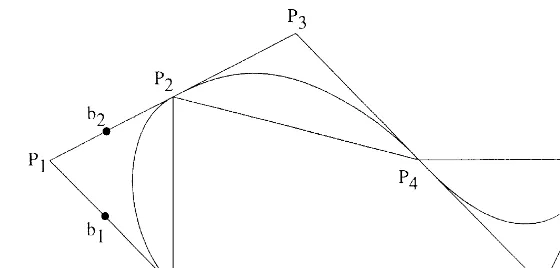
The curves described in this paper can protably be compared to rational quadratic Bezier curves and splines [4]. A quadratic Bezier curve is a conic arc in a control triangle. A spline created from them lies in a control polygon composed of triangles with collinear edges as in Fig. 1.
∗Corresponding author. E-mail: [email protected].
Fig. 1. AG2-cubic interpolating spline.
A particular conic arc within a triangle is usually determined by a weight w1, which controls how
far the curve is pulled toward the vertex, but could also be specied by giving a point inside the triangle that must be interpolated. Using conics however, there are only enough degrees of freedom to assign the curvature at one point of a spline. Also since a conic arc never has zero curvature, this prevents placing any inection points. Consequently G2-quadratic splines are of limited usefulness.
The curves to be studied here are similar to quadratic curves and splines in that we use the same control polygon, working in a sequence of triangles. This diers from the usual cubic control polygon that allows free placement of control points. Now b1 is restricted to lie on the segment P0P1 and b2 to lie on the segment P1P2 (see Fig. 1). The advantage of this is that it guarantees
that no inection point can occur in the interior of a triangle.
By using rational cubic Bezier curve segments in each triangle, we now have enough degrees of freedom to specify curvatures at both endpoints of every Bezier segment or every junction point of a spline. Furthermore, our construction allows the curvature to be set to zero at either or both ends of a curve segment. Thus an inection point can be inserted into a spline at a junction point, such as P4 in Fig. 1, but must be placed there purposely.
After the curvatures are set, the remaining degrees of freedom of the Bezier cubic within each triangle are controlled by two additional shape handles. The rst is a point B0 within the triangle that is interpolated. If B0 is constrained to the line joining P1 and the midpoint of P0P2, moving
it has the same eect as varying the weight w1 in the quadratic case. However as we shall see,
B0 cannot lie too near the vertex P1 if the curvatures at P0 and P2 are large. The second control
is by means of a slider that varies the curves through B0 within a family. The relationship of the
slider to the slope at B0 is observed to be monotonic most of the time, but the exact dependence is
not pursued in this paper. From the values given for these two shape handles, the locations of the control points b1 and b2 and the weights w1 and w2 are computed. The Bezier control points b0 and
b3 coincide with P0 and P2, respectively. The weights w0 and w3 have value 1.
These two controls are fully local in the sense that curvatures at the endpoints are not aected by them. The user can raise or lower the curve by movingB0 within the triangle and then slide through
the entire family of rational cubic Bezier curves that pass through B0 and join the endpoints with
prescribed tangents and curvatures.
at the ends and the singular point of the curve. These formulas are derived in Section 3. In Section 4 we see that the locus of singular points of Bezier curves with given interpolation conditions is a curve S of degree six. Certain arcs of S are composed of the singular points of cubics that are acceptable for modeling. These arcs are described in Section 5. Section 6 shows that the curve S
is birationally equivalent to a curve Q of degree 4. Using Q, in Section 7 we supply a proof of most of the claims made in Section 5 about arcs of S. Section 8 is devoted to the case in which one or both of the curvatures at the endpoints is zero. Section 9 contains some details related to programming and a summary.
2. Geometric preliminaries
A triangle P0P1P2 denes two systems of coordinates. The rst are barycentric for the ane plane.
The barycentric coordinates of a point P areP(s; t; u), wheres+t+u=1. The barycentric coordinates of the vertices of the triangle are P0(1;0;0), P1(0;1;0) and P2(0;0;1). The second coordinates are
homogeneous for the entire projective plane. The homogeneous coordinates ofP are P[s; t; u], written with square brackets. The only condition now on s; t; u is that they cannot all be zero. If P does not
lie at innity its homogeneous coordinates can be normalized to barycentric coordinates by dividing by s+t+u.
The following properties of an irreducible cubic are all equivalent [2]:
• It is rational, in the sense that it has a rational parametrization.
• It can be written as a rational Bezier cubic.
• It has genus zero.
• It is singular, with exactly one double point.
An implicit cubic curve that passes through P0 tangent to P0P1 and P2 tangent to P1P2 has an
as curvatures, although in reality they are only proportional to the true curvatures.
3. Formulas for the Bezier cubic
assigned barycentric coordinates b0(1;0;0), b1(X;1−X;0), b2(0;1−Y; Y) and b3(0;0;1). We refer
to X and Y as the control point ratios of b1 and b2.
Theorem 1. The formulas for the control point ratios X andY and the normalized weights w1; w2
(with w0=w3= 1) in terms of k0; k2 and the singular point B( s;t;u) are
Proof. There is a standard method for parametrizing the cubic F with singular point B [2]. Using
T as a parameter, the family of lines through B is given by
L(T) =T(ts−st) + (1−T)( ut−tu ) = 0:
Using resultants to eliminate rst s and then u between F and L(T), we obtain formulas for u=t and
s=t. When these are made homogeneous, we have a parametrization of F in terms of T:
s= (−su3+k2t
On the other hand, the standard Bezier parametrization of the same curve is
B(T) = (1−T)3w0(1;0;0) + 3T(1−T)2w1(X;1−X;0) + 3T2(1−T)w2(0;1−Y; Y)
w2=13[t( s(k0t
The formulas stated in the theorem for the weights are gotten by normalizing them so thatw0=w3=1
[7] or [4] and making some substitutions.
We will see in Section 7 that 06X; Y61 for our interpolating cubics. The formulas in Theorem 1 then show that w1 and w2 are nonnegative.
4. The singular point curve
With respect to the triangle P0P1P2 and curvatures k0 and k2, Eq. (1) takes the form
F=a(s2u
−k0st2) +b(su2−k2t2u) +estu−ft3= 0:
Modeling with these generally nonsingular curves is studied in [6].
Here we are interested in singular curves that have the form of F. The condition that F should have a specic double point B( s;t;u) is a linear condition in the coecients a; b; e and f. Solving
We see there is a unique cubic in our family with singular point B:
F= t3u(k2t
Another linear condition that can be imposed is that the cubic should interpolate a given point
B0(s0; t0; u0). Now the possible singular points are restricted to lie on the sextic curve
After rearrangement, the equation of this curve, the singular point curve, becomes
S=k0k2s0t0u0t6+ (k0s0u20−k0k2t20u0)st5+ (k2s20u0−k0k2s0t02)t 5u
−(s0u20−k2t02u0)s2t3u−(s20u0−k0s0t02)st3u2−t03s3u3
−(k0k2t03−2(k0+k2)s0t0u0)st4u+ 3s0t0u0s2t2u2= 0:
Theorem 2. The singular point curve is an elliptic curve of degree six that has triple points at P0
Proof. All of the rst partial derivatives of S vanish at B0 but not all the second derivatives do, so B0 is a double point. Similarly all the rst and second partials of S vanish at P0 and P2 but not all the third do, so these are triple points. To nd the tangent line(s) at the triple point P0(1;0;0), we
set s= 1 in S. The terms of lowest degree are the product of the expressions for the tangent lines at P0. In this case the lowest degree terms simplify to u3, so u= 0 is the only tangent line.
By resolving the singularity at P0 (or P2) as in [1], we nd the triple point P0 has an ‘innitely
near’ double point, or double point in its rst neighborhood. Thus it counts as (32) + (22) = 4 double points. Together, P0, P2 and B0 account for 9 double points. A sextic can have at most 10 double
points. The dierence 10−9 = 1 is the genus and so we have an elliptic curve. Another proof of this fact will follow from the construction in Section 6 of a birational transformation between the singular point curve and a quartic with two double points.
The cubic F and the singular point curve S are intimately related to each other, arising as they do from the same equation, but with the set of variables that is xed interchanged with the set that is not xed. Consequently a statement made about one curve has a corresponding statement about the other. For example,
(a) Given a cubic with singular point B, interpolating a pointB0, the singular point curve interpolates
B and has singular point B0.
Corresponds to
(a′) Given a singular point curve with singular pointB0, interpolating a point B, the cubic interpolates B0 and has singular point B.
A broader such pair of statements is:
(b) Given a cubic F with singular point B, each of its points B0 is the double point of a singular
point curve that has triple points at P0 and P2 and interpolates B.
(b′) Given a singular point curve S with double point B0, each of its points B is the singular point
of a cubic that has contact given by k0 and k2 at P0 and P2 and interpolates B0.
Statement (b′) is the foundation of this paper. We must investigate which segments of S correspond
to cubics with a geometrically reasonable arc inside the triangle. Then we need to parametrize these arcs of S so that we can easily move B along them. The formulas derived in Section 3 are then used to compute the control points and weights of the cubic that is determined.
5. Useful arcs of the singular point curve
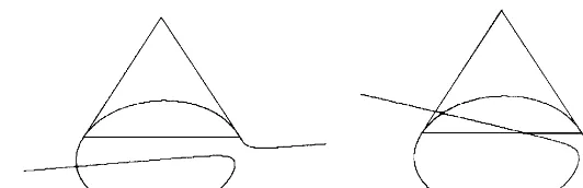
Not all of the cubics with singular point on S are acceptable for modeling purposes. A sampling of unacceptable curves is given in Fig. 2.
For the purposes of this paper, we dene a cubic to be good if it has a convex arc inside the triangle from P0 through B0 to P2 and if its singular point lies outside the triangle.
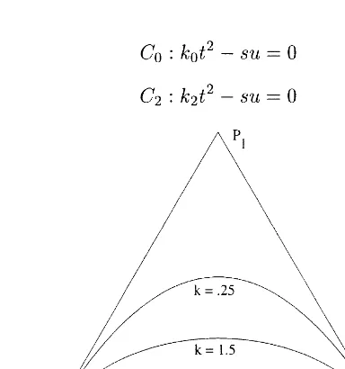
The curvatures k0 and k2 assigned at P0 and P2 determine two conics:
C0: k0t2−su= 0; C2: k2t2−su= 0:
These conics help delineate the regions in which B0 and B can lie in order for the cubic F to be
good. The larger the value of k0 or k2, the closer is the arc of the conic C0 or C2 in the triangle to
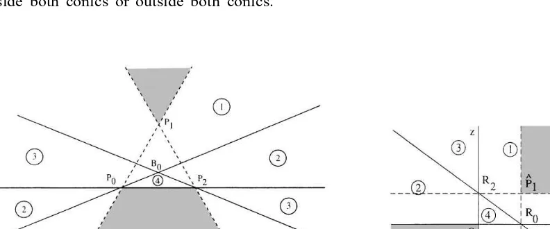
Fig. 2. Unacceptable curves that satisfy the contact conditions.
Fig. 3. Conics determined by curvatures.
The following theorem proves that there are two arcs of S that determine good cubics. In addition we will describe another arc of S, found experimentally, that determines cubics that do have a convex arc inside the triangle from P0 through B0 to P2, but that later reenter the triangle to cross
the rst arc. Although they are not good in our technical sense, these cubics are also acceptable for modeling since only the arc from P0 to P2 is used.
Theorem 3. If the interpolation point B0 lies in the interior of at least one of the two conics C0
or C2 then the singular point curve S has two arcs that determine good cubics. If B0 lies outside
both conics, there is no solution to the interpolation problem.
The theorem is proved Section 7. Here we illustrate where the arcs lie on S and what types of cubic we obtain. The description depends on whether B0 lies inside both conics, or lies inside one
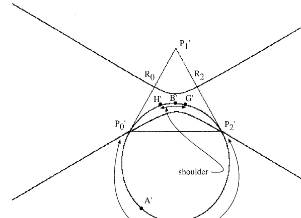
Fig. 4. The singular point curve forB0(0:35;0:3;0:35),k0= 0:25,k2= 0:3.
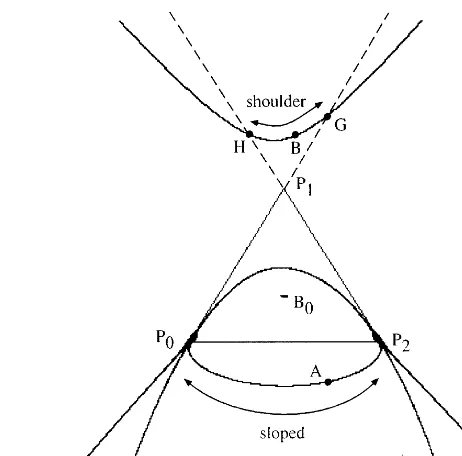
Fig. 4 shows an example of the singular point curve when B0 lies inside both conics; this is
detected by checking that both q0=k0t02−s0u0=C0(B0) and q2=k2t02−s0u0=C2(B0) are negative.
The interpolation point B0 is an acnode of S. The indicated arc from P0 to P2 consists of the
singular points of the sloped cubics. These curves have moderate-sized weights and are very useful for modeling. The sloped curve with singular point A is illustrated in Fig. 5.
The other arc between the points G[k2s0t0; q2;0] and H[0; q0; k0t0u0] on the lines u= 0 and s= 0
consists of the singular points of the shoulder cubics. These curves have fairly high weights. The shoulder curve with singular point B is also illustrated in Fig. 5.
Fig. 6 shows an example of the singular point curve when B0 lies between the two conics; in this example the curvature k0 is larger than k2. The loop based at P0 now determines the sloped cubics.
The arc that corresponds to shoulder cubics has stretched all the way to P2.
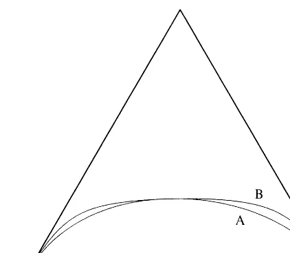
In addition to the arcs claimed in the Theorem, there is an additional arc that was discovered experimentally that gives useful cubics. It exists only when B0 lies between the two conics. The
arc itself lies inside the triangle, so the cubic has its double point inside the triangle. The third arc corresponds to the elbow curves, which naturally extend the family of sloped curves. The transition from sloped curve to elbow curve is illustrated in Fig. 7. All three types are illustrated in Fig. 8, but this time they are graphed as implicit curves rather than Bezier curves as in Fig. 5. Note the sloped curve A has an acnode at the point A, the elbow curve B has a crunode inside the triangle
at the point B, while the shoulder curve C has a crunode at the point C.
Fig. 5. Examples of sloped (A) and shoulder (B) cubics.
Fig. 6. The singular point curve for B0(0:35;0:3;0:35), k0= 1:5, k2= 0:3.
6. The quartic guide curve
In this section we show that the singular point curve S is birationally equivalent to a curve Q
Fig. 7. The transition from sloped curve to elbow curve.
Fig. 8. Examples of sloped (A), elbow (B) and shoulder (C) cubics.
Theorem 4. The singular point curve S is birationally equivalent to a curve Q of degree four.
(See Figs. 9 and 10:) The guide curve is an elliptic curve with double points at P′
0(1;0;0) and
P′
2(0;0;1). Its equation is
Q=−t04y4+s0t30xy 3+t3
0u0y3z+t0u0q2xyz2+s0t0q0x2yz+q0q2x2z2; (3)
where q0=k0t02−s0u0 and q2=k2t02−s0u0.
Proof. The following quadratic transformation transforms (s; t; u)-space to (x; y; z)-space.
x=t0t(t0u−u0t); y=t20su−s0u0t2; z=t0t(t0s−s0t):
The fundamental points where is not dened are P0, B0 and P2. The fundamental lines are
the three lines determined by these points. Away from these lines is invertible, and its inverse transformation −1 is given by
s=z(t0y−u0z); t=t0xz; u=x(t0y−s0x):
The fundamental points of −1 are R
0[t0; s0;0], P1′[0;1;0], and R2[0; u0; t0]. (For more information
about quadratic transformations, see [9].)
When the substitution−1 is made in the equation of the singular point curve we obtain the guide
curve. As before, partial derivatives are used to check the statements about double points.
Fig. 9. The guide curve corresponding to Fig. 4.
Fig. 10. The guide curve corresponding to Fig. 6.
The guide curves that are birationally equivalent to the singular point curves of Figs. 4 and 6 are illustrated in Figs. 9 and 10. The homogeneous coordinates of the transforms of G and H are G′[−q
2t0;−q2s0; s20t0] and H′[t0u20;−q0u0;−q0t0]. The arcs that correspond to the shoulder, sloped
and elbow curves are labelled. The transforms of A;B and C are also marked.
The guide curve can be made ane by setting y= 1 in (3); see Figs. 12–14. The ane guide curve is quadratic in each of x and z, so can be easily parametrized using one square root with either x or z as the parameter. By composing with −1 we obtain a parametrization for the singular
7. Proof of Theorem 3 and a Corollary
A cubic of the form (1) already crosses the line P0P2 twice, so by Bezout’s Theorem can cross it
at most once more. For a good cubic this third crossing cannot be in the segment P0P2; this means that the two coecients a; b of F must have the same sign, or that ab ¿0. We begin the proof by using this inequality to restrict the region of (s; t; u)-space in which B must lie. This in turn restricts
the region of (x; z)-space where we look for arcs of the ane guide curve. Working rst in (s; t; u)-space, the condition ab ¿0, together with (2), says
su(k0t 2
−su)(k2t 2
−su)¿0 (4)
from which it is easily seen that su must be positive, hence s and u have the same sign. Requiring
B to lie outside the triangle means t has the opposite sign. The shaded portions of Fig. 11(a) are
the regions of (s; t; u)-space to which B is restricted.
To determine the corresponding regions of (x; z)-space, we use the following easily determined facts about :
• P1 transforms to ˆP1(t0=s0; t0=u0). • s= 0 transforms to z=t0=u0.
• u= 0 transforms to x=t0=s0.
• t= 0 (a fundamental line) transforms to O(0;0).
Hence we can determine the images under of the four regions 1,2,3,4 determined by the fundamental triangle P0B0P2. Corresponding regions are numbered in Fig. 11(a) and (b) (ignore the
shading and dotted lines). Region 1 is split into four subregions by the dotted lines. The shaded region in Fig. 11(a) is bordered by t= 0, so corresponds to the shaded region in Fig. 11(b) with vertex at O(0;0).
In addition, we see from (4) that C0( B) and C2( B) must have the same sign. Thus B must either
be inside both conics or outside both conics.
The conics C0 and C2 transform via to conics in (x; z)-space:
G0=q0xz+s0t0x+t0u0z−t20;
G2=q2xz+s0t0x+t0u0z−t20:
Thus we are looking for the arcs of the guide curve that lie in the shaded region of Fig. 11(b) and either inside or outside both conics G0; G2.
The proof now splits into cases according to the signs and relative sizes of q0 and q2. The
following facts are used in the proof.
(a) The graph of Q(x; z) = 0 crosses the axes only at R0(t0=s0;0) and R2(0; t0=u0).
(b) The curve Q(x; z) = 0 crosses the line z=t0=u0 exactly twice: simple intersections at R2 and at
(−t0u0=q0; t0=u0).
(c) The curve Q(x; z) = 0 crosses the line x=t0=s0 exactly twice: simple intersections at R0 and at
(t0=s0;−s0t0=q2).
(d) The curve Q= 0 intersects each Gi= 0 in exactly two nite points, R0 and R2.
(e) As a polynomial of degree two in z,
Q(x; z) =A(x)z2+B(x)z+C(x);
where
A(x) =q2x(t0u0+q0x); B(x) =t0(t02u0+s0q0x2); C(x) =t03(s0x−t0):
The guide curve Q can be solved for z in terms of its discriminant x(Q) =B(x)2−4A(x)C(x):
z1=−
B−√x(Q)
2A ; z2=
−B+√x(Q)
2A :
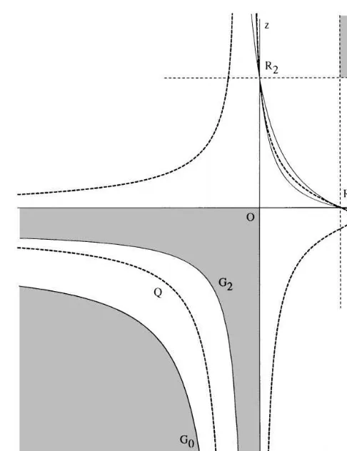
Case 1. Assume that B0 lies in the interior of both conics C0 and C2, and in particular that
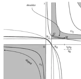
q2¡ q0¡0. Fig. 12 shows the shaded region of the (x; z)-plane in which we are searching for arcs
of the guide curve, and the guide curve itself which appears dotted. We will see that there are exactly two arcs of z1= 0 in the shaded region and no arcs of z2.
For x ¡0, −AC ¿0, so that √x(Q) is real. Because
√
x(Q)¿|B(x)|, z1¡0 but z2¿0. The
graph of z1 in the third quadrant therefore determines good cubics–the sloped cubics.
For x∈(t0=s0;−t0u0=q0), again −AC ¿0, so that √x(Q) is real, z1¿0 and z2¡0. We see
immediately that the graph ofz2 does not enter the shaded region. Forx in this interval we need to see
that the graph ofz1 lies abovez=t0=u0 and below the graph of G2. Usingz1(t0=s0) =−s0t0=q0¿ t0=u0
and z1(−t0u0=q0) =t0=u0 and assertion (b) we see that the graph of z1 lies above z=t0=u0 in this
interval. Furthermore, since the vertical asymptote of G2 occurs at x=−t0u0=q2, which is inside the
x-interval, and by (d) the graphs of Q and G2 do not cross in the interval, the graph of z1 lies
below the graph of G2. This arc of Q= 0 determines the shoulder cubics. It can not be extended
past x=−t0u0=q0 because the graph of z1 has crossed the line z=t0=u0.
Also for x ¿−t0u0=q0, the graph of z2 lies between the two conics. To see this, consider the two
equalities
(q2xz+t02)G0−Q=−t03xz(k2−k0)(t0−s0x); (5)
Fig. 12. The ane guide curve (dotted) forB0(0:3;0:4;0:3); k0= 0:4; k2= 0:2.
At a point ofQ= 0 for whichx ¿−t0u0=q0 and z ¿ t0=u0 the right side of the rst is negative, while
the right side of the second is positive. At the same time, q0xz+t02 and q2xz+t02 are both negative.
So G0(x; z) and G2(x; z) must have opposite signs, and the graph of z2 lies between the two conics.
The proof in the case q0¡ q2¡0 is the same for x ¡0. For x∈(t0=s0;−t0u0=q0) the graphs of
G0 and G2 are interchanged and one shows that the graph of z1 lies below the graph of G0.
Case 2. Now assume that B0 lies between the two conics C0 and C2, and in particular that
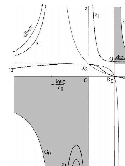
q2¡0¡ q0. Fig. 13 shows the shaded region of the (x; z)-plane in which we are searching for
arcs of the guide curve, and the dotted guide curve. Again we will see that there are two arcs of
z1= 0 in the shaded region that correspond to the sloped and shoulder arcs. In addition, the arc that
corresponds to the elbow cubics is labelled; it also is part of the graph of z1.
For x∈(−t0u0=q0;0),
√
x(Q) is real, z1¡0 and z2¿0. The graph of z1 in this interval is the
arc of Q= 0 that determines the sloped cubics. It cannot be extended for x ¡−t0u0=q0, for there
both z1; z2¿0 (although one of these arcs determines the elbow cubics).
For x∈(t0=s0;∞), again −AC ¿0, so that √x(Q) is real, z1¿0 and z2¡0. Using z1(t0=s0) =
−s0t0=q0¿ t0=u0 and assertion (b) we see that the graph of z1 lies above z=t0=u0 in this interval.
And for the same reason as in case 1, the graph of z1 lies below the graph of G2. The graph of z1
over this interval is the arc of Q= 0 that determines the shoulder cubics.
To conclude this case, we have to consider the situation q0¡0¡ q2. The proof is similar, except
Fig. 13. The ane guide curve (dotted) forB0(0:3;0:4;0:3); k0= 1; k2= 0:1.
Case 3. Finally assume that B0 does not lie inside either conic C0 or C2, and in particular that
0¡ q0¡ q2. We will see there are no arcs of Q= 0 in any of the zones of the (x; z)-plane shaded
in Fig. 14.
We start by checking that the intersection of the guide curve with the shaded zone in the rst quadrant is empty. After performing the substitution x=r+ (t0=s0); z=w+ (t0=u0) in Eq. (3) for
Q= 0, we see that every sign in the resulting equation is positive. Hence there are no solutions for
r ¿0 and w ¿0.
Next consider the third quadrant and again use Eq. (5). For points in the third quadrant, the right hand side of the rst is negative while that of the second is positive, while the coecients of G0
and G2 are positive. Hence no points of Q= 0 satisfy G0G2¿0.
Now that we have obtained arcs of the ane guide curve on which ab ¿0, we must check that this is sucient to guarantee that the points determine good cubics. By construction the singular points of the cubics lie outside the triangle. Next we show that the cubic crosses into the triangle at no points other than P0 and P2. In order that the cubic does not cross between P0 and P1 we need
c and f, therefore a and f to have the same sign, or af ¿0. Similarly we need bf ¿0. Thus in addition to (4) we want
−st(k2t 2
−su)(k0k2t 4
−s2u2)¿0;
−tu(k0t 2
−su)(k0k2t 4
Fig. 14. The ane guide curve (dotted) for B0(0:3;0:4;0:3); k0= 2; k2= 4.
Recall we are working at points where s;u have the same sign opposite to that of t. Note that when
k0t 2
−su and k2t 2
−su have the same sign, k0k2t 4
−s2u2 also has this sign. So inequality (4) implies both of these two inequalities. Hence a cubic entering the triangle at P0 must leave at P2,
and being the only segment of the cubic in the triangle, must pass through B0 on the way. That
the arc is convex follows from the variation diminishing property, once we have established the following corollary.
Corollary. For good cubics, the control point ratios satisfy
06X; Y61:
Proof. The proof uses the fact that for any real numbers a and b,
0¡ a
a+b¡1 if and only if ab ¿0:
For X this is used with a=−k2tC 0( B) and b= uC2( B). Then
ab=−k2tuC 0( B)C2( B)
8. The case of curvature zero
In this section we study what happens when one or both of k0 or k2 is zero.
The shoulder curves tend to have fairly large weights anyway, but as the curvature k0 tends to
zero, the weight w1 on that side tends to innity. The limiting shoulder cubic whenk0=0 factors into
the product of the lineu= 0 and a conic. Similarly when k2= 0 the cubic factors into the product of
the line s= 0 and a conic. When both k0 andk2 equal zero, the cubic factors as the product of three
lines. Because of their tendency to have large weights and the fact that they are reducible when a curvature equals zero, the shoulder cubics are perhaps less useful for modeling than the sloped and elbow cubics. The sloped and elbow curves have more moderate weights and do not all become reducible if k0 and/or k2 equals zero. These curves can be used to introduce inection points where
needed in splines.
However, we must discuss three situations for sloped and elbow cubics when k0 and/or k2 is zero:
• one of k0; k2 is zero but the other is not, and B0 lies inside both conics,
• one of k0; k2 is zero but the other is not, and B0 is between the two conics,
• both of k0; k2 are zero, in which case B0 necessarily lies inside both (reducible) conics –
anywhere in the triangle.
First if k2= 0, k06= 0 and q0=k0t20−s0u0¡0, B0 is inside both conics. There are sloped curves
but no elbow curves. The guide curve factors
Q= (t0−u0z)(−t03+s0t02k0x2z+s0t02x+s0t0u0xz−s20u0x2z)
(see Fig. 15). If we choose x ¡0 we can easily compute z. The cubic that corresponds to the point
A is the intermediate curve graphed in Fig. 16.
If k2= 0 and q0¿0, B0 lies between the two conics. A typical graph of the guide curve appears
in Fig. 17. The intersection point I is
t0(−s0u0−t0
To the left of I the corresponding cubics are reducible and are no longer useful solutions to our
interpolation problem. Thus the parameter domain, forx in this case, must be restricted to (t0(−s0u0−
t0
√
s0u0k0)=s0q0;0).
When both k0 and k2 equal zero, the guide curve factors
Q= (t0−u0z)(t0−s0x)(s0u0xz−t02)
(see Fig. 18). The cubic in Fig. 19 that corresponds to A has zero curvature at both ends.
When either or both curvatures are zero, some modications are needed in the formulas in Theorem 1. If k0= 0 then Y = 0, so the control point b2=P1. Similarly if k2= 0, X = 0, so that b1=P1. In
either of these cases the formulas given for w1 and w2 fail, as there are zeros in the denominator.
However the formulas for w1 and w2 can be thought of as depending on X=k2 and Y=k0. It is easy
to nd the limit of Y=k0 as k0−→0, so this formula can be substituted instead to nd the formulas
Fig. 15. The ane guide curve for B0(0:35;0:3;0:35), k0= 0:3,k2= 0.
Fig. 16. The range of cubics with curvature zero atP2;B0(0:35;0:3;0:35); k0= 0:3,k2= 0.
Fig. 18. The ane guide curve for B0(0:35;0:3;0:35), k0= 0,k2= 0.
In this section we go through several other details that must be managed in a program to produce the sloped and elbow cubics. Then we give the pseudocode for graphing one adjustable curve arc in a xed triangle.
It is reasonable to constrain the location of B0 to the line segment joining the midpoint of triangle
Table 1
Bezier curve. However, B0 must not be permitted to go above the taller of the two conics. If a curvature is changed so that the taller conic moves down, when it reaches B0 it must pushB0 down
with it.
When q0¿0 the negative x-axis is divided by an asymptote at x=−t0u0=q0 into the domain for
elbow curves and the domain for sloped curves; see Fig. 13. Similarly when q2¿0 the negative
z-axis is divided by an asymptote at z =−s0t0=q2. Since we must select x and compute z when
q0¿0, and select z and compute x when q2¿0, it is reasonable to switch from selecting x when
k0 is greater than k2, to selecting z when k2 becomes greater than k0. Of course when one of q0; q2
becomes positive it is also necessary to test for the asymptote after selecting x or z.
As we saw in the proof of Theorem 3, the good cubics for k0¿ k2 were determined by points
on the graph of z1, never z2. For k2¿ k0, the correponding function x1 is used. Table 1 summarizes
the formulas and the domains for the three types of cubic: The functions x1 and z1 are the following:
where
We now give the pseudocode for one curve arc. The number appearing is a small positive constant.
Pseudocode for sloped and elbow cubics
initialize screen display of triangle and default B0(s0; t0; u0)
initialize sliders for k0; k2;B0 and the guide curve, all in [0,1]
{interpret the B0-slider as the distance from the midpoint M of P0P2
to the intersection of P1M and the taller of the two conics}
initialize a Flag to x or z, to indicate whether the guide curve slider is currently being used to select x in (−∞;0] or z in [0;−∞)
graph the default curve
main loop: whenever a slider is moved
if the B0-slider, move B0 and recompute (s0; t0; u0)
if the k0 or k2 slider, move the B0-slider if necessary to reect the true location
of B0 with respect to the taller conic, or if B0 is now above the taller conic,
set the B0-slider to 1, move B0 and recompute (s0; t0; u0)
if the guide curve slider,
set q0=k0t02−s0u0 and q2=k2t02−s0u0
if (q2¿0)
if (Flag=x) {k2 was jumped ahead. Expect a discontinuous jump in the curve}
reinitialize guidecurveslider and set Flag=z {choose z next time} set z=guidecurveslider/(guidecurveslider-1) {choose z in [0;−∞)} set I =t0(−s0u0−t0
√
s0u0k2)=u0=q2
if (k0= 0) and (z ¡ I) set z=I + {don’t let z get smaller than I}
if (|t0s0+q2z|¡ ), z=z+ {avoid the asymptote}
set x=x1(z; q0; q2)
else if (q0¿0)
if (Flag=z) {k0 was jumped ahead. Expect a discontinuous jump in the curve}
reinitialize guidecurveslider and set Flag=x {choose x next time} set x=1-1/guidecurveslider {choose x in (−∞;0]}
set I =t0(−s0u0−t0
√
s0u0k0)=s0=q0
if (k2= 0) and (x ¡ I) set x=I+ {don’t let x get smaller than I}
if (|t0u0+q0x|¡ ), x=x+ {avoid asymptote}
set z=z1(x; q0; q2)
else if (k2¿ k0) and (Flag=x) {k2 just became larger than k0}
set x=1-1/guidecurveslider {choose x one last time} set z=z1(x; q0; q2)
set Flag=z{choose z next time} set guidecurveslider=z=(z−1)
else if (k0¿ k2) and (Flag=z) {k0 just became larger than k2}
set z=guidecurveslider/(guidecurveslider-1) {choose z one last time} set x=x1(z; q0; q2)
set Flag=x{choose x next time} set guidecurveslider=1=(1−x) else if (Flag=x)
set x=1-1/guidecurveslider set z=z1(x; q0; q2)
else {Flag=z}
set z=guidecurveslider/(guidecurveslider-1) set x=x1(z; q0; q2)
from x and z compute ( s;t;u) on the singular point curve compute X and Y
compute w1 and w2 depending on whether k0= 0 and/or k2= 0
graph the curve end main loop
References
[1] S. Abhyankar, Algebraic Geometry for Scientists and Engineers, Mathematical Surveys and Monographs, vol. 35, Amer. Math. Soc., Providence, RI, 1990.
[3] C. de Boor, K. Hollig, M. Sabin, High accuracy geometric Hermite interpolation, Comput. Aided Geom. Design 4 (1987) 269–278.
[4] G. Farin, Curves and Surfaces for Computer Aided Geometric Design, Academic Press, New York, 1993.
[5] T. Goodman, K. Unsworth, Shape preserving interpolation by curvature continuous parametric curves, Comput. Aided Geom. Design 5 (1988) 323–340.
[6] M. Paluszny, R. Patterson, Geometric control ofG2-cubic A-splines, Comput. Aided Geom. Design 15 (1998) 261– 287.
[7] R. Patterson, Projective transformations of the parameter of a Bernstein–Bezier curve, Comput. Aided Geom. Design 4 (1985) 276–290.