Crime, coordination, and punishment
An economic analysis
Peter-J. Jost*
WHU-Otto-Beisheim-Hochschule, Institute for Organization Theory, Burgplatz 2, D-56179 Vallendar
Abstract
In the standard economic theory of crime and punishment, a risk-neutral individual will commit an offense if and only if his private benefit exceeds the expected sanction for doing so. To the extent that several individuals simultaneously choose whether or not to commit the offense, it is assumed that their decisions are independent of each other.
The purpose of this paper is to investigate a situation in which an individual’s propensity to engage in an illegal activity may depend also on the behavior of other individuals. We consider a two-period model: In each period, individuals decide simultaneously whether to commit the offense. A police authority is in charge for the arrest and conviction of offenders. We assume that the police authority has a limited enforcement budget such that it cannot arrest and convict every offender. In this situation, the expected payoff of an individual from committing the offense is higher the more individuals also decide to behave illegally.
We analyse the interactive behavior in this model and answer the following questions: When are individuals responding to others’ behavior, when are they influencing others’ behavior. And, what is the optimal enforcement policy to forestall interactive behavior. © 2001 Elsevier Science Inc. All rights reserved.
1. Introduction
In Basel, Switzerland, handicrafts are traditionally organized in guilds. Besides represent-ing the interests of their members, the main purpose of guilds is to share business information and to cultivate commercial relations. Commenting on enforcement of environmental reg-ulations, representatives of the environmental agencies in Basel remarked that meetings by
* Corresponding author. Tel.: 49-261-65-09-300; fax: 49-261-65-09-111. E-mail address: [email protected] (P.-J. Jost).
guild members are also used to exchange information concerning individual compliance with law. They expect that such information about the behavior of other members influences the propensity of one member to comply with environmental regulations.
The reason for this apprehension is well justified: To induce as many firms as possible to engage in adequate protection, the environmental agencies used a sequential enforcement process—see for example Shavell [1991] or Mookherjee and Png [1992]: First, they make spot inspections (general enforcement) which keeps enforcement costs low, but implies that monitoring will be imprecise. If a monitoring visit indicates insufficient protection, an agency investigates in a second step the actual degree of the firm’s protection at high cost (specific enforcement). Now suppose that the owner of an environmentally risky plant knows that others are already violating environmental regulations. Since a limited enforcement budget restricts the agency’s ability to detect all violations, the agency has to concentrate its specific enforcement activities to only some of those firms where general enforcement indicated an offense. But then the incentive of the owner to behave illegally increases with the number of firms already violating the regulations because the probability that the agency actually investigates his plant decreases.
One of the most important issue confronted by environmental agents thus is to organize their enforcement activities to forestall such interactive behavior. The standard literature on crime and punishment fails to give a suitable theoretical answer to this issue. According to Becker’s [1968] seminal study, a risk-neutral individual will commit an offense if and only if his private benefit exceeds the expected sanction for doing so.1To the extent that several individuals simultaneously choose whether or not to commit the offense, it is assumed that their decisions are independent of each other. An individual’s compliance decision then is not influenced by the behavior of other individuals. The behavior of the aggregate is merely an extrapolation from the behavior of an individual.
Situations, however, in which an individual’s behavior depends on what others are doing usually do not permit simple extrapolation of individual behavior to the aggregate.2To make that connection we then have to look at the system of interaction between individuals: When do individuals respond to others’ behavior; when do they influence others’ behavior; and (in case of criminal activities) what is the optimal enforcement policy to forestall interactive behavior?
The purpose of this paper is to investigate these questions in a game-theoretical model.3
1
See e.g. Ehrlicher [1973], Becker and Landes [1974], Heinecke [1978], Andreano and Siegfried [1980], Pyle [1983], Schmidt and Witte [1984] or the symposium on the economics of crime in the Journal of Economic Perspectives Vol. 10(1) [1996] and the references therein.
2
Empirical evidence on tax evasion, for example, suggests that evasion decisions are not independent. Instead, individuals are more likely to evade once they expect others evading; see e.g. Benjamini and Maitail [1985], Schlicht [1985] or Gordon [1989]. This interactive behavior is also common to many other criminal or social activities; see Case and Katz [1991]. For instance, one’s incentive to double-park is higher if many others do so and one is less discouraged from smoking marijuana if most of one’s friends do. The formation of mobs, riots, or panic behavior are other examples. See Schelling [1978, p. 36ff] for a more elaborate discussion.
3
There are two risk-neutral individuals. Each individual knows his own private benefit from committing an offense, but not the other individual’s payoff. The timing of the game has two periods. In each period, individuals decide simultaneously whether to commit the offense. An offender is subject to a sanction when he is caught. Before his second period decision, an individual observes the first period behavior of the other individual. A police authority is in charge of the arrest and conviction of offenders in both periods. We assume that the police authority has a limited enforcement budget such that it cannot arrest and convict every offender per period.4 In this situation, interactive behavior emerges because the expected sanction for an offender if both individuals commit the offense is lower than the expected sanction if only one individual commits the offense. As a result, the expected payoff to an individual from committing the offense is higher the more likely it is that the other individual is also an offender.5
The first issue with interactive behavior in our model lies on the supply side of offenses. Because of their interdependent payoff functions, an individual must anticipate the behavior of the other. In the two period model, an individual will use the first period behavior of the other individual as a signal of his propensity to engage in the illegal activity at date two. Of course, to be (or not to be) an offender in period one is not a commitment to future behavior. This introduces coordination problems. Since both individuals prefer to coordinate their decision to commit the offense, the following two behavior patterns may arise: In case of active coordination, an individual commits the offense at date one in order to demonstrate high private benefits but switches to legal behavior at date two if the other individual behaved legally at date one. And, in case of passive coordination, an individual behaves legally at date one and switches to illegal behavior at date two if the other individual committed the offense at date one.
The second issue relates to the demand side of offenses, i.e. the way police authority should allocate resources for policing between the two periods. The way in which police resources are allocated influences the possibility for interactive behavior of individuals and therefore the overall crime rate. We assume that the authority’s objective is to minimize the total number of offenses in both periods.6 To this purpose, it will try to reduce possible coordination between individuals.
In Section 2 we introduce into the basic one-period model. In the next two sections we analyze the two-period model. First, in Section 3, we consider the case in which the
analyzes a dynamic relationship in which an individual’s current information concerning the probability of punishment is influenced by past experiences of the individual and of his acquaintances. Chu concentrates on a special class of interactions characterized by the model of critical mass.
4
From a normative point of view, police should have the budget that maximizes social welfare, see e.g. Polinsky and Shavell [1999]. In the positive analysis of law, however, it is common to assume that the enforcement budget is set by legislative in a general budget process and therefore given for an enforcement agency, see Stigler [1970] or Jost [1997]. See also footnote 7.
5
These network externalities are analyzed in the industrial organization literature, see e.g. Farrell and Saloner [1985, 1986] or Katz and Shapiro [1985, 1986]. In this literature, however, it is assumed that an individual’s decision in period 1 is a commitment for his behavior in period 2.
6
police authority has a fixed identical budget for each period. This case captures the features of many enforcement problems in reality and focuses only on interactive behavior under a given institutional framework. Second, in Section 4, we analyze the general case in which the police authority has the possibility to shift part of its budget from one period into another period.7 We characterize individuals’ behavior for any given allocation of resources and then show how the authority should allocate resources optimally in order to minimize the expected number of offenses. Section 5 concludes with some final remarks.
2. The one-period model
There are two risk-neutral individuals. Both have to decide simultaneously at date 1 whether or not to commit an offense. Let O, respectively N, denote the decision (Not) to commit the Offense. An individual’s benefit from engaging in the illegal activity is denoted by i [ [0, 1]; i is his private information and is independently drawn from the uniform distribution on [0, 1].8If an individual does not commit the offense, his benefit is normalized to zero.
A police authority is in charge of the arrest and conviction of offenders. It uses the following sequential enforcement process:9 First, spot inspections indicate some evi-dence whether an individual has committed the offense or not. Without loss of generality we assume that these general enforcement activities involve no costs. Spot inspections provide enough information for the police authority to fully concentrate on a guilty person. However, because of the impreciseness of spot inspections, the police authority is required to provide sufficient evidence about the offense in order to arrest and convict an offender. Since its enforcement budget is limited the authority can investigate only one offender. If it investigates, then with some probability, p [ [0, 1], the offender’s behavior is perfectly revealed and with some probability, 1 2 p, the behavior is not
7
Note, that the authority’s objective function puts a zero weight on the benefits of offenses. This is reasonable, if the social value of offense is arbitrarily negativ. In general, the authority should maximize the net surplus of an offense. See e.g. Garoupa [1999] who proposes that organized crime could improve social welfare.
8
Once the coordination problem is analyzed, it would be straightforward to take the enforcement and the sanction as endogenous and solve for the socially optimal budget and the optimal sanction using backwards induction.
9
The assumption that private benefits are uniformly distributed allows us to concentrate our analysis on the question, in which circumstances the individuals’ interaction between two periods results in a coordination of criminal behavior. In particular, this assumption ensures that there is a unique equilibrium in the one-period model, see Result 1. That is, there are no coordination problems between individuals within each period.
revealed. The authority chooses the probability of detection p such that its total enforce-ment budget is used. If an individual’s behavior is not revealed, that individual is not convicted. If, however, an offender’s behavior is revealed, he is arrested and convicted and has to pay a sanction F. F is assumed to be fixed and lower than one, F[[0, 1]. Its budget as well as the sanction is exogenously given.
The sanction an offender has to expect then depends on the behavior of the other individual; i.e., individuals’ payoff functions are interdependent.10To commit an offense is more beneficial to an individual the higher the probability that the other individual behaves illegally. In fact, letp(i, s; s9) denote the expected payoff to an individual with
benefit i if he chooses action s[{N, O} and the other individual chooses action s9[{N,
O}. Then
p~i, N; s9!50 for s9 [{N,O},
p~i, O; N!5i2pF
p~i,O;O!5i2pF/ 2.
In the following, let f denote the expected sanction for an individual who committed the offense if the other individual also engaged in the illegal activity, i.e. f 5 pF/ 2.
To analyze individuals’ behavior, we define an equilibrium strategy profile as a function
s* :@0,1#3S5$N,O%
such that s*(i) maximizes the expected payoff of an individual with private benefit i, i[
[0, 1], given the other individual with benefit j, j [ [0, 1], chooses the strategys*( j).11 That is,
s*~i!5argmax
s[S
E
0 1
p~i,s;s*~j!!dj.
Result 1: There exists a unique equilibrium strategy profile s* with the following
properties: Let i*s 5f/(1 2 f ). Then an individual with benefit i less than i*s does not commit the offense, whereas an individual with a benefit higher than this critical value decides to commit the offense. That is,
s*~i!5
H
N if i,i*s,O otherwise.
10
Of course, the coordination problem in the one-period model is a simple coordination game. In principle, experimental economics can here be used to make predictions about the behavior in these games, see e.g. van Huyck, Battalio and Beil [1990].
11
To prove this result, suppose that an individual with benefit i decides to commit the offense. Then an individual with a higher benefit j$i will behave in the same way. Similarly, if an
individual with benefit i decides not to commit the offense, an individual with a lower benefit
j #i will not engage in the illegal activity. Hence, there exists a critical value i*s such that
individuals with higher (lower) benefits choose (not) to commit the offense. The individual with benefit i*s then must be indifferent between the two choices. That is,
05i*
s~i*s22f!1~12i*s!~i*s2f!, hence i*s 5 f/1 2 f.
3. The two-period model without budget shifting
In the two-period model, individuals decide simultaneously in each period whether or not to commit an offense. If an individual commits the offense, he enjoys his benefit i but may be sanctioned for his behavior. After period 1 each individual observes the behavior of the other individual.12At date 0, a police authority coordinates its enforcement activities for both periods. We assume in this section, that the police authority has an identical limited enforcement budget for each period. Budget shifting from one period into another period is not possible. Hence, the probabilities of detection p1 in period 1 and p2 in period 2 are identical, p1 5 p2 5 p.
Each individual has eight possible strategies in the two-period model:
s1 5(N, N) : do not commit the offense at date 1 and 2;
s2 5(N, O) : do not commit the offense at date 1 but do commit the offense at date 2;
s3 5(O, N) : commit the offense at date 1 but not at date 2;
s4 5 (O, O) : commit the offense at date 1 and at date 2;
s5 5 (N, OuO) : do not commit the offense at date 1 and commit the offense at date 2 only if the other individual behaved illegally at date 1;
s6 5(N, OuN) : do not commit the offense at date 1 and commit the offense at date 2 only if the other individual behaved legally at date 1;
s7 5 (O, OuO) : commit the offense at date 1 and commit the offense at date 2 only if the other individual behaved illegally at date 1; and
s8 5 (O, OuN) : commit the offense at date 1 and commit the offense at date 2 only if the other individual behaved legally at date 1.
12
Let S 5 {s1, . . . , s8}. For a given strategy profile s: [0, 1] 3 S let dk denote the probability that an individual chooses action sk. Then an individual with benefit i [[0, 1] has the following payoff when choosing sk (with f 5 pF/ 2):
p(i, s1;s) 5 0 p(i, s
2;s) 5 (d2 1 d4 1d6 1 d8)(i 2f ) 1 (d1 1 d3 1d5 1 d7)(i 2 2f )
p(i, s
3;s) 5 (d3 1 d4 1d7 1 d8)(i 2f ) 1 (d1 1 d2 1d5 1 d6)(i 2 2f )
p(i, s
4;s) 5 p(i, s3;s) 1 (d21d41d51d7)(i2f )1(d11d31d61d8)(i22f )
p(i, s
5;s) 5 (d4 1 d8)(i 2f ) 1 (d3 1 d7)(i 22f )
p(i, s
6;s) 5 (d2 1 d6)(i 2f ) 1 (d1 1 d5)(i 22f )
p(i, s7;s) 5 p(i, s3;s) 1 (d4 1d7)(i 2f ) 1 (d3 1d8)(i 22f ) p(i, s8;s) 5 p(i, s3;s) 1 (d2 1d5)(i 2f ) 1 (d1 1d6)(i 22f )
An equilibrium for the two-period model without budget shifting then is a functions*: [0,
1] 3 S 5 {s1, . . . , s8} such that for every i [ [0, 1]
s*~i!5argmax
s[S
E
0 1
p~i, s; s*~j!!dj.
Consider an individual with private benefit i $ 2f. His payoff when committing an
offense is positive regardless of the decision of the other individual. Since his benefit would be zero if he would decide not to commit the offense, he will choose strategy (O, O). Thus, in every equilibriumd4 $ 1 22f. On the other hand, an individual with a low benefit i ,
f will never commit the offense. He plays (N, N) since if he failed to do so, his expected
payoff would be negative. Thus,d
1 $ f in every equilibrium.
Now consider an individual whose private benefit is in the intermediate range [ f, 2f]. First, we claim that it can never be optimal for him to commit the offense at date 2 if the other individual behaved legally at date 1. That is, (N, OuN) or (O, OuN) cannot be equilibrium
strategies. Intuitively, this result rests on the fact that in our model individuals want to conform and not to be different; both individuals prefer to coordinate their illegal activity. Since a legal behavior in period 1 indicates low private benefits, it is likely that this individual behaves legally also in period 2. Thus, committing the offense in response to a legal behavior cannot be optimal.
be used when deciding on the behavior in the second period. In equilibrium, of course, an individual uses the full conditional probabilities in making inferences about the other individuals’s likely second period behavior. In sum, these arguments motivate the following result:
Result 2: For any equilibrium s*[, the strategies (N, OuN), (O, OuN), (N, O), and
(O, N) cannot be equilibrium strategies for any individual.
An immediate consequence of this result is that an individual’s propensity to engage in the illegal activity is directly correlated with private benefit. The higher the private benefit, the greater the property to engage in the illegal activity. To confirm this, we have simply to compare the expected payoff when choosing different strategies. Because an individual with a sufficiently low, resp. high, benefit decides to choose strategy (N, N), resp. (O, O), i.e. d1 and d4 are strictly positive, simple calculation
shows that for an individual with benefit i [ [ f, 2f]
i~p~i, sk;s*!2p~i, sl;s*!!.0 for sk
5~O, O!, ~O, OuO! and s
l5(N,N), (N,OuO). Hence, the incentive to commit the offense in period 1 is greater the higher the private benefit to an individual. To see that this monotonicity property is also true for the second period decision, it remains to be shown that the expected payoff difference between playing strategies (N, N) and (N, OuO), resp. (O, OuO) and (O, O), is positively correlated with
the benefits. Simple calculation and the fact that the probability to commit the offense at date 2 increases from zero (when playing strategy (N, N)) to d4 1 d7 [ (0, 1) (when playing
strategy (N, OuO) or (O, OuO)) up to one (when playing strategy (O, O)) then proves the
following result:
Result 3: Every equilibriums*[has the following monotonicity properties:
1. If an individual with private benefit i [ [0, 1] decides to commit the offense at date 1, every individual with a higher benefit i9 $ i also commits the offense at date 1.
2. The probability that an individual commits the offense at date 2 is higher the greater his private benefit i [ [0, 1].
We now characterize individuals’ behavior in equilibrium. According to our previous results, any equilibrium involves the strategies (N, N) and (O, O) and may involve the strategies (N,
OuO) or (O, OuO). Note first that there is always an individual with private benefit in [ f, 2f]
for whom neither (N, N) nor (O, O) is optimal. For purposes of argument, suppose this is false. Then there exists an individual who is just indifferent between these two strategies (according to Result 1, his private benefit is determined by f/1 2 f ). His expected payoff
is zero. But then this individual benefits from deviating to strategy (N, OuO). Because he can
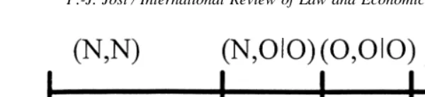
Case 1: Active coordination
Suppose that strategy (N, OuO) is not played by any individual. In this situation an
individual either chooses strategy (N, N), (O, OuO) or (O, O). We call this situation active coordination since an individual who chooses (O, OuO) commits the offense in the first
period in order to signal his propensity to engage in the illegal activity in the second period. In fact, as we will see, although his overall expected payoff is positive, his expected first period payoff is negative. The corresponding strategy profile s[is shown in Figure 1.
An individual with benefit i1then is indifferent between strategies (N, N) and (O, OuO) if
05~12i
1!~i12f!1i1~i122f!1~12i1!~i12f!,
which implies i1 5 1 2 =1 2 2f. Indifference between strategies (O, OuO) and (O, O) for an individual with benefit i2 requires
~12i
1!~i22f!5~12i1!~i22f!1i1~i222f!,
which implies i2 5 2f. To show that this strategy profile actually forms an equilibrium, it remains to be proven that no individual with benefit i [[i1, i2] has an incentive to deviate from his equilibrium strategy by choosing (N, OuO). According to Result 3, it is sufficient
to show that an individual with benefit i1 cannot benefit by deviating. But this is true, since his expected payoff would be negative, equal to2(1 2 i2)(i1 2 f ).
Case 2: Passive coordination
Suppose that strategy (O, OuO) is not played in equilibrium. Then only the strategies (N, N), (N, OuO) and (O, O) are part of a potential equilibrium. We call this situation passive coordination since an individual who chooses strategy (N, OuO) only engages in an illegal
behavior (at date 2) if he is sure that the other individual will do so. Note that if he observes
Fig. 1. Active coordination.
an offender at date 1, he knows with certainty that this individual repeats the offense at date 2. The strategy profiles[in this case is shown in Figure 2.
An individual with benefit i1then is indifferent between strategies (N, N) and (N, OuO) if
05~12i
2!~i12f!,
which implies i1 5 f. Moreover, an individual with benefit i2 is indifferent between strategies (N, NuN) and (O, O) if
~12i
2!~i22f!5~12i2!~i22f!1i2~i222f!1~12i1!~i22f!1i1~i222f!, which implies i2 5 f 1 (=1 1 8f
2
2 1)/ 2. This strategy profile constitutes an equilib-rium, if no individual has an incentive to deviate to strategy (O, OuO). Consider an
individual with benefit i2. If he deviates to strategy (O, OuO), his first period payoff has to be negative. According to Result 1, this is satisfied only if his private benefit i2 is lower than the critical value i*s. In fact, p(i2, s7; s) is lower than p(i2, s5; s) if and only if (1 2
i2)(i2 2 f ) 1 i2(i2 2 2f ) is negative, hence, i2 has to be lower than f/1 2 f. Using the characterization of i2, his property is satisfied if f is sufficiently high, that is f . (3 2 =5)/ 2.
Case 3: Active and passive coordination
Finally, consider the case in which (N, OuO) as well as (O, OuO) are part of an
equilibrium. The strategy profiles[then is shown in Figure 3.
Calculation shows that indifference between the strategies (N, N) and (N, OuO) at i 5
i1 between (N, OuO) and (O, OuO) at i 5 i2 and between (O, OuO) and (O, O) at i 5 i3 imply the following system of equations:
05~12i3!~i12f!1~i32i2!~i122f! (1)
05~122i
21i3!~i22f!1~2i22i3!~i222f! (2) 05~i
22i1!~i32f!1i1~i322f! (3)
Here, an individual with benefit i2 must have a negative first period payoff from com-mitting the offense in period 2. This is because his second period payoff when choosing (O,
OuO) is higher than when playing (N, OuO). Using strategy (O, OuO) he signals his
propensity to engage in the illegal behavior in period 2. This increases the incentive of the other individual to also behave illegally at date 2. A negative first period payoff when choosing (O, OuO) then implies that i2 has to be lower than the critical value i*s.
Moreover, an individual with benefit i3 must have a positive first period payoff from engaging in the illegal activity. Otherwise, he could benefit from choosing strategy (N,
OuO). Therefore, i3 must be higher than i*s.
Similar to the situation studied in case 2, the condition i2 , i*s requires that the penalty
f has to be higher than the critical value f . (3 2 =5)/ 2. This ensures that the expected first period payoff for an offender at date 1 is negative. To see this, consider the limit case in which i2 tends to i3; the above strategy profile then reduces to the equilibrium profile in case 2 and i2 becomes f 1 (1 2 =1 1 8f
2
)/ 2. Moreover, equation (2) then implies that
i2 5 f/1 2 f. Since i2 is positively correlated with f, i2 is lower than i*s only if f 2(1 2
=1 18f2)/ 2 , f/1 2 f which is equivalent to f . (3 2 =5)/ 2.
Result 4: The two-period model without budget shifting has the following equilibria:
– For f [ [0, 3 2 =5/ 2],
4. The general two-period model with budget shifting
In this section, we assume that the police authority is free to decide which part of its budget to use for detection in period 1 or 2. It will choose a partition of its budget in order to minimize the expected number of offenses. As before, the overall enforcement budget is limited such that the authority cannot police individuals with certainty in every period.
Let ( p1, p2) [[0, 1] 2
be the probabilities of detection in period 1 and 2 such that total budget is used. Define fi5 piF/ 2 as the expected sanction for an offender in period i, i5 [1, 2], if the other individual also commits the offense. Then ( f1, f2) [ [0, 1/ 2]
2
following, we consider ( f1, f2) as the police authority’s policy variables. Limited budget then restricts the police to f1 1 f2 # B for some B [ [0, 1].
As in Section 3, let S5{s1, . . . , s8} denote the possible strategies for an individual and letd
kdenote the probability that an individual plays strategy sk. For a given strategy profile
s: [0, 1] 3 S, an individual with benefit i [ [0, 1] then has the following payoff when
choosing strategy sk:
p(i, s1;s) 5 0
p(i, s2;s) 5 (d2 1 d4 1d6 1 d8)(i 2f2) 1 (d1 1 d3 1d5 1 d7)(i 22f2) p(i, s3;s) 5 (d3 1 d4 1d7 1 d8)(i 2f1) 1 (d1 1 d2 1d5 1 d6)(i 22f1) p(i, s4;s) 5 p(i, s3;s) 1 (d2 1 d4 1 d5 1 d7)(i 2 f2) 1 (d1 1 d3 1 d6 1 d8)
(i 2 2f2)
p(i, s5;s) 5 (d4 1 d8)(i 2f2) 1 (d3 1d7)(i 22f2) p(i, s6;s) 5 (d2 1 d6)(i 2f2) 1 (d1 1d5)(i 22f2)
p(i, s7;s) 5 p(i, s3;s) 1 (d4 1d7)(i 2f2) 1(d3 1d8)(i 22f2) p(i, s8;s) 5 p(i, s3;s) 1 (d2 1d5)(i 2f2) 1(d1 1d6)(i 2 2f2)
An equilibrium for the two-period model with budget shifting is a triple ( f *1, f *2,s*) with
s*: [0, 1] 3 [0, 1/ 2]2 3 S such that
– for a given policy ( f1, f2)
s*~i; f
1, f2!5
argmax
s[S
E
0 1
p~i, s; s*~j!!dj,
for every individual with beneift i [ [0, 1] and
– the policy ( f *1, f *2) minimizes the expected number of offenses over all policies ( f1, f2) with f1 1 f2 # B.
To analyze the model, we first consider the behavior of individuals in response to the police authority’s policy choice ( f1, f2). Similar to the argument in Section 3, it can be shown that it is never optimal for an individual to choose strategy (N, OuN) or (O, OuN).
In either case, an individual would commit the offense in response to a legal behavior of the other individual, although this indicates low private benefits and, hence, a low propensity of the other individual to commit the offense in period 2. In contrast to Result 2, however, it may now be optimal for an individual to choose strategy (N, O), resp. (O, N); if, for example, there is no policing at date 1, resp. date 2, an individual commits the offense regardless of his private benefit.
Moreover, as in the two-period model without budget shifting, it is straightforward to show that individuals’ incentives to engage in the illegal activity are greater the higher the private benefits. If an individual with benefit i commits the offense at date 1, then an individual with a higher benefit i9 . i will do so; and, the probability that an individual will
be an offender at date 2 is greater the higher his private benefit.
An immediate consequence from this monotonicity result is that the strategies (O, N) and (N, O), resp. (N, OuO), cannot be part of the same equilibrium strategy profile s*. To see
i, resp. i9. Monotonicity in the propensity to commit the offense in period 1 then requires i.
i9. Monotonicity in period 2, however, requires i ,i9, a contradiction. Similarly, it is easy to show that (N, O) and (O, OuO) are not optimal strategies for individuals in the same
equilibrium profile.
With these remarks we are now in the position to characterize the equilibrium strategy profile s*(z, f
The proof of Result 5 can be found in the Appendix as well as the characterization of the critical values x1, . . . , x4and i1, i2, respectively i3, for each strategy—they are well defined functions of f1 and f2. Two remarks are worth noting. First, x2 is lower than x3 if and only if f1 1f2 is lower than some critical value around 0.618. In this case, there exists for every
possible equilibria for f1 [ [ x3, x2]. Second, x4 is lower than 1/2 if f1 1 f2 is lower than =3/2 50.866. If this is not the case, the strategy profile s*5 is never played.
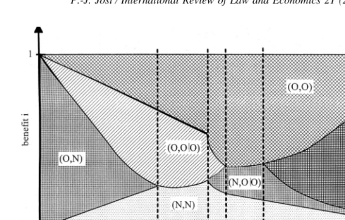
Figure 4 provides an example of the unique equilibrium strategy profile in the case where
f1 1 f2 5 1/ 2 (that is, the authority can police individuals with certainty in one of the two periods and the sanction F is one):
Of course, if there is no policing at date 1, i.e. f15 0, an individual commits the offense regardless of his private benefit. However, the expected penalty f2 5 1/ 2 ensures that no individual repeats his offense at date 2 (see Result 1). If the police authority now increases its policing in period 1 and reduces proportionally its policing in period 2, individuals with low benefits will not commit in either period but those with high benefits will be offenders in both periods. Moreover, it becomes profitable for some individuals to coordinate actively; they commit the offense in the first period in order to signal their propensity to engage in the illegal behavior in the second period. If the first period expected sanction f1 exceeds the critical value x1, playing strategy (O, N) is no longer optimal. Since the second period sanction f2 is sufficiently low, the probability that an offender repeats his offense is sufficiently high. However, if the first period sanction f1 increases further, active coordina-tion becomes less attractive. If f1 then is greater than the critical value x2, some individuals will switch to passive coordination. They do not commit the offense in the first period, but do so in the second period if the other individual committed the offense in the first period, but do so in the second period if the other individual committed the offense in the first period. Passive and active coordination become more, resp. less, attractive to individuals the higher the first period sanction f1. In fact, if this sanction becomes sufficiently high, f1 $ x3, no individual will coordinate actively. When the first period sanction f1 then becomes higher and, therefore, the second period sanction f2 becomes lower, the incentive to commit the offense at date 2 becomes higher. If f1$x4it is then optimal for some individuals to choose
strategy (N, O). In the limit, if there is no policing in period two, an individual commits the offense at date 2 regardless of his benefit. However, since f151/ 2 in this case, no individual will be an offender at date 1 (see Result 1).
Having characterized the individuals’ behavior in response to a policy choice ( f1, f2) of the police authority, we now consider how police actions should be coordinated in both periods when the enforcement budget is limited such that f1 1 f2 # B. The example above suggests the following result: whenever the police authority is in action with certainty in one period, there is no offense in this period, but both individuals commit the offense in the other period. In this situation, an individual cannot learn anything about the actual benefit of the other individual. That is, his ex post probability distribution at date 2 on the other’s benefit is identical to his ex ante probability distribution at date 1. This, however, is no longer true if the police authority decides to police in both periods; in this case, there is a positive probability that an individual coordinates his second period decision on the observed behavior of the other individual in the first period. Hence, an individual has better information on the other individual’s benefit at date 2 than at date 1. This increases his incentives to behave illegally, either in period 1 by signaling his propensity to commit the offense also in the second period or in period 2 as a response to the illegal behavior of the other individual in period 1. As a consequence, the expected number of offenses will be higher than in a situation in which no coordination is possible.13
Result 6: In the two-period model with budget shifting, it is optimal for the police
authority to choose the following policing strategy ( f *1, f *2):
– If B [ [0, =3/ 2], then
f*15
H
B if B,1/ 2,1/ 2 otherwise f*25
H
0 if B,1/2,
B21/2 otherwise
as well as f*15
H
0 if B,1/ 2,
B21/ 2 otherwise f*25
H
B if B,1/2, 1/2 otherwise minimizes the expected number of offenses which are
42 2B
12B for B,1/ 2, resp. 42
4
322B for B$1/ 2.
– If B [ [=3/ 2, 1], then f*151/ 2, f*25B21/ 2
minimizes the expected number of offenses which are
13
42 4
322B.
The proof of Result 6 can be found in the Appendix. The result can be reconciled with the intuitive argument discussed before: it is optimal for the police authority to minimize coordination between individuals. As a consequence, the police authority should be in action in one of the two periods with maximal probability. It is unimportant whether this is done in period 1 or 2, as long as the enforcement budget is not too high. In fact, the strategy profiles
s*1 and s*5 always lead to the same number of expected offenses. However, as Result 5 shows, if B exceeds the critical value =3/2, the strategy profile s*5 is no longer an equilibrium strategy profile. Instead,s*4now describes the optimal individuals’ behavior for maximal detection in period 1. Buts*4allows more coordination than s*1.
5. Conclusion and extensions
In this article we have analyzed decision-interdependency among potential offenders and characterized the optimal enforcement policy to forestall interactive behavior. We have shown that it is optimal for a police authority to concentrate police actions in order to minimize coordination between individuals.
To the extent that there are more than two periods, this result suggests that it is optimal for the police authority to use the following strategy: concentrate resources in period 1 to forestall criminal behavior, and do so in all subsequent periods as long as the budget allows. This, of course, is a well known strategy in real law enforcement situations. For example, local transport companies often use surprise controls with several ticket inspectors to avoid interactive travelling without a ticket.
Our result could also be extended to different types of offenses.14Suppose for example that there are two types of offenses and that the police authority has a limited budget to enforce both offenses. If the authority is free to allocate its resources, our results suggest the following optimal policing strategy: concentrate police actions on one type of offense in period 1 and on the other type of offense in period 2. If, however, the police authority is restricted in its allocation of resources, conditional policing in period 2 is optimal: shift as many resources as possible to the enforcement of that offense, that is most prevalent in period 1.
We assumed throughout the paper that the police authority can commit itself to a certain policy. Therefore, individuals (when deciding on whether to commit the offense) can condition their behavior on this information. Although this is a standard assumption in the theory of crime and punishment (see Besanko and Spulber [1989] for an exception), it would be of interest to consider a situation in which the police authority decides on policing
14
simultaneously with the individuals’ decisions. The literature on tax evasion suggests that the optimal policing crucially differs from the one derived here, see e.g. Reinganum and Wilde [1985, 1986]. In particular, if the tax authority cannot commit itself to its auditing policy, it faces the following credibility problem: Suppose that from an ex-ante perspective, the tax authority prefers to audit with positive probability, thus providing appropriate incentives for truthfully given tax reports. However, if the taxpayers behave as supposed, the tax authority might not have an ex-post incentive to audit, for it can save on costs. Of course, his behavior will be foreseen by the taxpayers and the authority’s ex-ante announcement to audit will not be credibly ex-post. Thus, the tax authority has to rearrange the tax system in such a way that his threat to audit becomes credible at the time of performance.15
The model could also be extended to consider the case in which the authority is required partially to self-finance by retaining a share of the sanctions it collects. Further work should also consider more than two individuals. The mechanism discussed here may then serve as an explanation of the formation of riots and mobs.
Acknowledgment
I am grateful to Martin Hellwig, the editor of this journal and two anonymous referees for helpful suggestions and comments. Financial support by the Stiftung Mensch-Gesellschaft-Umwelt (MGU) at the University of Basel is gratefully acknowledged.
Appendix
Proof of result 2
Lets* be an equilibrium strategy profile. We distinguish four cases:
1. Consider first the case of strategy s65(N, OuN) and suppose that s6is part ofs*. Then there exists an equilibrium in whichd
6is strictly positive. Hence, there exists a range in [ f, 2f] such that an individual with private benefit in this range chooses strategy s6. Let j [[ f, 2f] be the individual with the lowest benefit j such that s6is his equilibrium strategy profile. Since strategy s15(N, N) yields zero payoff, the individual with benefit j must have at least a non-negative payoff, that is
p~j, s
6;s*!5~d21d6!~j2f!1~d11d5!~j22f!$0. (1) We now argue to a contradiction: we show that j must be greater than 2f, which implies thatd
6 50, since an individual with benefit greater than 2f prefers to choose strategy (O,
O) in equilibrium.
15
To prove this, let j 5 tf for t[ [1, 2]. Suppose that it is optimal for an individual with benefit i [ [ f, 2f] to play strategy s2 5 (N, O). Then we claim that it cannot be optimal for an individual with a higher benefit i9 $i to play strategy (N, OuN). To see this, note that d
4 is strictly positive. Hence,
i~p~i, s2;s*!2p~i, s6; s*!!.0.
and the incentives to play s2 5(N, O) instead of s6 5 (N, OuN) are greater the higher the
individual’s benefit. In particular, j,i. As a consequence, the probability that an individual
plays strategy s2 or s6 is less than f(2 2 t). That is, d2 1 d6 , f(2 2 t).
Since d1 $ f and p6( j, s6; s*) is an increasing function of d2 and d6, but is also a
decreasing function ofd1andd5for j[[ f, 2f], inequality (1) then implies that (with t5tn)
f~22t
n!~j2f!1f~j22f!.0, that is j.tn11f with tn115 42tn
32t
n .
Then tn11 . tn and in the limit,
j. lim
n3`
42t
n 32t
n
zf52f, a contradiction.
2. Consider now the case of strategy s85(O, OuN). As before, suppose thatd8.0. Let
j[[ f, 2f] be the lowest benefit to an individual for whom it is optimal to play strategy s8. Then p( j, s8; s*) must be higher than p( j, s3; s*) which implies that
~d
21d5!~j2f!1d1~j22f!$0.
Similar to the argument in part one of this proof it follows that j . 2f, a contradiction. 3. Suppose thatd
2.0. Let j [ [ f, 2f] be the lowest benefit to an individual for whom it is optimal to play strategy s2 5 (N, O). Thenp( j, s2;s*) must be higher than p( j, s5;
s*) which implies that
d
2~j2f!1~d11d5!~j22f!$0.
Sinced2 ,f and d1 1d5 $ f, an argument similar to part one of this proof shows that
j . 2f, a contradiction.
4. Suppose that strategy s3 5 (O, N) is played by some individuals, that isd3.0. We distinguish two cases:
4.1. Suppose thatd5.0. Sinced1is strictly positive, the incentives to play strategy s35
(O, N) instead of strategy s5 5 (N, OuO) are greater the higher the individual’s benefit,
i~p~i, s3;s*!2p~i, s5; s*!!.0.
Moreover, since
it follows that there exists a critical value i1 [[ f, 2f] such thatp(i1, s3; s*)5 p(i1, s5;
s*). This implies
~d
31d7!f5~d11d5!~i122f!.
Since i1 ,2f, the right hand side of this equation is negative, whereas the left hand side is positive, a contradiction.
4.2. Suppose thatd550. Then the equilibriums*[consists of the strategies s1, s3, s7,
s4. To see thatd7.0, note that p(i, s3;s*) 2 p(i, s2;s*) 5 ad7 is independent of an individual’s benefit i. Sinced3 .0 and s2 5 (N, O) cannot be part of the equilibrium,d7
must be strictly positive. According to part 4.1, it is optimal for an individual with benefit i[ [ f, 2f] to play strategy s7 and it cannot be optimal for an individual with a higher benefit i9
$ i to play strategy s3.
An individual with benefit i1 then is indifferent between strategies s1and s3 if i15f/12
f (see Result 1) and an individual with benefit i2 is indifferent between strategies s3 and s7 if 0 5 (1 2 i2)(i2 2 f ) 1 (i2 2 i1)(i2 2 2f ). Hence,
The monotonicity property ensures that there exist three critical values i1, i2, i3 such that
p~i
1, s1; s!5p~i1, s3;s!,
p~i
2, s3; s!5p~i2, s7;s!,
p~i3, s7; s!5p~i3, s4;s!.
Simple calculation shows that these equations imply
x1 12x
1
5B2x
1.
Note that if there is no first period sanction, f1 50, an individual commits the offense at date 1 regardless of his private benefit, i.e. i1 5 0 and does so at date 2 if his benefit is sufficiently high, i.e. i2 5 f2/1 2 f2.
Case 2: (N, N), (O, OuO) and (O, O) are part of a strategy profile
In this case there exist two critical values i1, i2, such that
p~i1, s1; s!5p~i1, s7;s!,
p~i
2, s7; s!5p~i2, s4;s!. These equations are equivalent to
05~12i1!~i12f1!1i1~i122f1!1~12i1!~i12f2!
05i
1~i222f2!
The solutions for i1 and i2 can be easily calculated as
i15 2
22f
11f2
2 2
Î~2
2f11f2!224~f11f2!2 , i252f2.
Now, the first equation implies that i1$f2for otherwise (O, N) would yield a higher payoff than (O, OuO). But then the expected first period payoff must be negative, that is i1 #
f1/1 2 f1. Therefore, a necessary condition for (s1, s7, s4) to constitute an equilibrium strategy profile is f1 $ x1.
In addition, the strategy (N, OuO) must result in a negative payoff for an individual with
benefit i1. This condition is equivalent to
~12i
2!~i12f2!1~i22i1!~i122f2!#0.
If it holds, i1 is lower than 2f2 which ensures that i1 , i2, since the second equation implies i2 5 2f2. Moreover, this condition is satisfied for f1 5 x1: the left hand side then is identical to 2( f2)
2
. However, if f2 is sufficiently small, the left hand side becomes positive. Hence, there exists a critical value x2 , 1/ 2, x2 . x1, such thatp(i1, s5; s) # 0 for all f1 # x2. In fact, x2 is the smallest solution of the identity (1 2 i2)(i1 2 (B 2
x2)) 1 (i2 2 i1)(i1 2 2(B 2 x2)) 5 0 with
i15
21B22x2
2 2
Î~2
1B22x2!224B2 , i252~B2x2!.
Case 3: (N, N), (N, OuO) and (O, O) are part of a strategy profile
In this case two critical values i1, i2, exist such that an individual with benefit i1 is indifferent between choosing strategies (N, N) and (N, OuO), i.e.p(i
1, s1;s) 5 p(i1, s7;
Strategy (N, O) yields a lower payoff than (N, OuO) for an individual with benefit i2 if
i2(i2 22f2) is negative, i.e. i2 ,2f2. Moreover, strategy (N, OuO) is more profitable than
(O, OuO) if
~12i2!~i22f2!1i2~i222f1!#0.
This inequality is satisfied if and only if i2# f1/12f1. In addition, the second equation implies
where x3 is the smallest solution of the identity
x3
and x4 is the smallest solution of the identity
2x45 21
Three remarks are worth noting. First, x4 is strictly greater than x3 for all B [ [0, 1]. Second, x3is strictly lower than 1/2 for all B[[0, 1]. Third, x4is higher than
1
Case 4: (N, N), (N, OuO), (O, OuO) and (O, O) are part of a strategy profile
An individual with benefit i1 is indifferent between strategies (N, N) and (N, OuO), an individual with benefit i2 is indifferent between (N, OuO) and (O, OuO), and an individual with benefit i3is indifferent between (O, OuO) and (O, O) if the following three equations are satisfied:
05~12i
3!~i12f2!1~i32i2!~i122f2! 05~12i
2!~i22f1!1i2~i222f1!1~i32i2!f2 05i
1~i32f2!1~i22i1!~i32f2!
This system of equations requires that i1 . f2 and i3 , 2f2. Note that if i1 is identical to i2, the system of equations reduces to the one studied in case 2 and if i2is identical to i3, it reduces to the one studied in case 3. The range in which the strategy profile (s1, s5, s7,
s4) then constitutes an equilibrium profile depends on the critical values x2 and x3: If x2 ,
x3, the profile is an equilibrium strategy profile for f1 [ [ x2, x3]. If, otherwise, x2 . x3, it is an equilibrium profile for f1 [ [ x3, x2]. Note that x2 . x3 implies multiplicity of equilibrium profiles. This occurs if F is higher than some critical value around 0.617. Note that although 0.617 is lower than 32 =5, this result is in line with Result 2: as long as B is lower than 32 =5, 32 =5/2 is lower than x3 and, hence, is not within the interval [ x3,
x2]. For B 5 3 2 =5 we then have x3 5 3 2 =5/ 2.
Case 5: (N, N), (N, OuO), (N, O) and (O, O) are part of a strategy profile
In this case there exists an individual with benefit i1 who is indifferent between choosing strategies (N, N) and (N, OuO), i.e.p(i1, s1;s)5p(i1, s7;s), an individual with benefit i2who
is indifferent between (N, OuO) and (N, O), i.e.p(i2, s7;s)5p(i2, s2;s) and an individual with
benefit i3who is indifferent between strategies (N, O) and (O, O), i.e.p(i2, s2;s)5p(i2, s4;s).
These three critical values are solutions of the following system of equations:
05~12i3!~i12f2!
05~i
32i2!~i22f1!1i2~i222f1! 05~12i
3!~i32f1!1i3~i322f1!1~i22i1!f2
The first and the second equations imply i15f2and i25i3f2/i32f2. Hence i1,i2. Using the characterization for i2, the condition i2 #i3is satisfied if and only if i3$2f2. Since for i2 identical to i3 the system of equations reduces to the one studied in case 3, this condition is equivalent to f1 $x4. Note that the third equation also implies that i3#f1/12f1. Q.E.D.
Proof of result 6
V15422i1~11i3!22i2~12i1!
V25422i
1~22i11i2!
V35422i
1~12i2!22i2~11i3!
V45422i1~12i2!22i2~11i2!
V55422i1~12i3!22i3~11i2!
Using the characterization of the critical values i1, i2, resp. i3(see the proof of Result 5), calculation shows that V1 is increasing in f1 and V2, V3, V4 and V5 are decreasing in f1. Since the strategy profiles*iis identical to the strategy profiles*i11for f15xi, xias defined in the proof of Result 5, the expected number of offenses then is minimal for f150 or f25 0. The claim of Result 6 then follows immediately. Q.E.D.
References
Andreano, R., & Siegfried, J. (1980, eds.). The economics of crime, New York: Wiley.
Becker, G. (1968). Crime and punishment: an economic approach. Journal of Political Economy, 76, 169 –217. Becker, G., & Landes, W. (1974, eds.). Essays in the economics of crime and punishment, New York: Columbia
Univ. Press.
Benjamin, Y., & Maital, S. (1985). Optimal tax evasion and optimal tax evasion policy: Behavioral aspects. In W. Gaetner and A. Wenig (eds.): The economics of the shadow economy, Berlin: Springer.
Besanko, D., & Spulber, D. F. (1989). Delegated law enforcement and noncooperative behavior. Journal of Law, Economics, and Organization, 5, 25–52.
Boadway, R., Marceau, N., & Marchand, M. (1996). Time-consistent criminal sanctions. Public Finance, 149 –165.
Case, A., & Katz, L. (1991). The company you keep: The effects of family and neighborhood on disadvantaged youth. NBER Working Paper No. 3705.
Chu, C. (1993). Oscillatory vs. stationary enforcement of law. International Review of Law and Economics, 13, 303–315.
Ehrlicher, I. (1973). Participation in illegitimate activities: a theoretical and empirical investigation. Journal of Political Economy, 81, 521–565.
Farrell, J., & Saloner, G. (1986). Standardization, compatibility, and innovation. Rand Journal of Economics, 16, 70 – 83.
Farrell, J., & Saloner, G. (1986). Installed base and compatibility: innovation, product preannouncements, and prediction, American Economic Review, 76, 940 –955.
Garoupa, N. (2000). The economics of organized crime and optimal law enforcement. Economic Inquiry, 38(2), 278 –288.
Gordon, J. P. (1989). Individual morality and reputation costs as deterrents to tax evasion. European Economic Review, 33, 797– 805.
Heineke, J. (1978, ed). Economic models of criminal crime, Amsterdam: North-Holland.
Jost, P. J. (1997). Monitoring, appeal, and investigation: the enforcement and legal process. Journal of Regulatory Economics, 12, 127–146.
Katz, M., & Shapiro, C. (1985). Network externalities, competition, and compatibility. American Economic Review, 75, 424 – 440.
Kydland & Prescott (1977). Rules rather than discretion: the inconsistency of optimal plans. Journal of Political Economy, 85, 473– 491.
Mookherjee, D., & Png, I. (1992). Monitoring vis-a-vis investigation in enforcement of law, American Economic Review, 82, 556 –565.
Polinsky, A., & Shavell, S. (1999). The economic theory of public enforcement of law, NBER Working Paper No. 6993.
Pyle, D. (1983). The economics of crime and law enforcement, New York: St. Martin’s.
Reinganum, J., & Wilde, L. (1985). Income tax compliance in a principal-agent framework. Journal of Public Economics, 26, 1–18.
Reinganum, J., & Wilde, L. (1986). Equilibrium verification and reporting policies in a model of tax compliance. International Economic Review, 27, 739 –760.
Sah, R. (1991). Social osmosis and pattern of crime. Journal of Political Economy, 99, 1272–1296. Schelling, T. (1978). Micromotives and macrobehavior, New York: Norton.
Schlicht, E. (1985). The shadow economy and morals: a note. In W. Gaetner and A. Wenig (eds.): The Economics of the Shadow Economy, Berlin: Springer.
Shavell, S. (1991). Specific versus general enforcement of law. Journal of Political Economy, 99, 1088 –1108. Shavell, S. (1992). A note on marginal deterrence. International Review of Law and Economics, 12, 345–355. Stigler, G. (1970). The optimum enforcement of laws. Journal of Political Economy, 78, 526 –536.