*Corresponding author. Tel./Fax:#39-6-725-97358. E-mail address:[email protected] (A. D'Angelo).
Production variability and shop con
"
guration: An
experimental analysis
Andrea D
'
Angelo!
,
*
, Massimo Gastaldi", Nathan Levialdi#
!Department of Production, Systems and Computer Science, University of Rome-Tor Vergata, Italy
"Department of Electrical Engineering, University of L'Aquila, Italy
#Department of Industrial Engineering, University of Perugia, Italy
Received 6 June 1998; accepted 4 February 1999
Abstract
The selection of an e$cient shop layout at manufacturing level is a strategic problem, involving considerable
immobilisation of"nancial resources. Often the problem is hierarchically solved on several levels. In the present paper we
focus on the level of physical system planning and try to de"ne the best shop con"guration in terms of process resources
layout (work centres organisation), considering di!erent variability conditions for demand (system input). Data obtained
from simulation experiments are being statistically analysed to clear the weak and strong points for each con"guration
(job shop,#exible cell shop,#ow shop). ( 2000 Elsevier Science B.V. All rights reserved.
Keywords: Manufacturing systems; Shop layout; Simulation; Performance evaluation; Production variability
1. Introduction
The selection of an e$cient productive layout at manufacturing level is a strategic problem, involv-ing considerable immobilisation of "nancial resources. Therefore, planning and design of pro-duction lines include a careful analysis [1], devoted to individuate technological bind that the related production imposes, factors in#uencing strategic system performances and the opportune tool for the selection of the best solution. Often the problem is hierarchically resolved on several levels. In par-ticular, the level of physical system planning re-quires a further distinction of physical components
from the control logic. In the present paper we focus on the "rst item: organisation of process resources layout. The manufacturing layout choice passes in fact through the quanti"cation of trade-o! between routing #exibility and set-up savings, i.e., performances of alternative con"gurations showing symmetric advantages and disadvantages. In particular, the analysis goes over a restricted set of alternative choices: job shop, cellular manufac-turing,#ow shop and hybrid systems. The"rst type is a process layout and involves a system resource organisation in isolated work centres, in which machines perform all the same type of processing on parts to be produced. The second type of layout is organised in isolated cells in which only a suit-ably scheduled product family is processed. That is, system resources are allocated at di!erent working departments on the basis of technological binds
imposed by production cycle of products families. The third type of layout provides the organisation of dedicated production #ow lines in which part types follow obliged and unidirectional routes. Be-sides there exist other hybrid forms which mediate functional features of the two types just described. The attractiveness of each type of con"guration is basically tied to the particular system performance considered by management. Aim of this research is to compare alternative productive layouts testing their robustness with respect to system input varia-bility. That is, we want to quantify trade-o! between routing#exibility and set-up savings with respect to di!erent condition of demand variability. Such variability will be modelled through the vari-ation coe$cient of lots inter-arrival time to the system and through unbalancing of product mix. Simulation experiments will be conducted with this aim: gathering the correlation between system per-formances and such experimental factors testing the relative statistical signi"cance.
The paper is organised as follows: in Section 2, literature contributions are reviewed aiming to underline the main topics investigated in this research area. In Section 3, the system under study is brie#y described, while in Section 4, the paper's aims are presented in terms of research questions, experimen-independent factors and the observed dependent variable. Data obtained by simulation experiments are analysed in Section 5 and "nally Section 6 concludes the paper discussing the major results and possible future research issues.
2. Relevant literature review
In literature, works that investigate dynamics related to productive#ows in a manufacturing sys-tem agree in recognising the process layout to be superior in terms of e$ciency performance. Morris and Tersine [2] proved that the job shop has the best performance in almost all experimental test conditions. Observed system performances (mean throughput time and the work in process inven-tory) are analysed with respect to a series of test factors such as demand stability, productive #ow direction and set-up time. Statistical analysis con-ducted on experimental results data shows that
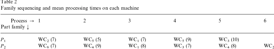
Table 2
Family sequencing and mean processing times on each machine
ProcessP 1 2 3 4 5 6
group technology and cellular manufacturing. Ang and Willey [8] stated that group technology and hence cellular manufacturing lacks the #exibility necessary for coping with work-load variations. They concluded that this choice is not always eco-nomically justi"ed in practice. Also Leonard and Rathmill [9], although formerly proponents of group technology, believed good process layout would prove superior in comparison with cellular layout shop con"guration.
3. System description
In the above contributions, production system was assigned through a more or less complex part-machine matrix. Here this matrix was randomly generated (Table 1).
To this purpose, the following assumptions were made:
f total number of possible processing (6); f total number of product families (4);
f minimum and maximum number of operations
expected for each product family (3}6);
f minimum and maximum value of cycle time
rela-tive to each processing for each kind of part type (5}10 minutes).
In generating the part-machine matrix we do not impose the condition of unidirectional#ow, i.e., it is possible for a part type to be processed by a ma-chine visited before. Such an hypothesis was con-sidered important for a more realistic adhesion. It introduces a complication which is partly balanced by the extreme easiness of the part-machine matrix. Results of the random formulation are reported in Table 2. For each family the manufacturing cycle sequencing is shown in terms of visited machines (the mean value of cycle time for each operation). As you can see, part familyP2undergoes six opera-tions, whileP4only three. Moreover, only manu-facturing cycle sequencing forP4does not involve backward processing, since its cycle provides operations on all di!erent machines. To this pur-pose parts belonging to product family P
2 have a double reprocessing: its cycle involves passage on machines 4 and 6, in two di!erent situations.
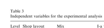
Table 3
Independent variables for the experimental analysis
Level Shop layout Mix I-a variability
0 Job shop Balanced Null
1 Flexible cell shop Medium unbalanced Medium 2 Flow shop Strongly unbalanced Large
is 0.2). Moreover it is assumed that all machines are subject to breakdown events. For each server allo-cated in a work centre, these events have a prob-ability occurrence distributed in a log-normal curve around a mean value of 1000 minutes and a stan-dard deviation of 100 minutes. Mean time to repair, instead, is distributed in a Gamma curve with a mean value of 50 minutes. Parts to be produced arrive at the system in lots of "xed size (5). In designing work centres, cells or#ow lines, in terms of minimum server allocation necessary to respect the continuity bound and to avoid system parts' accumulation, we make use of the following model [10,11]:
505is the hourly total system input,;mis the
average expected utilisation, C
j is the percentage
mix relative to familyj(j"1,2, 4) and¹p ijis the
average processing time for parts belonging to fam-ilyj, for operationi.
Total system load is balanced by the production capacity of each centre, cell or line, given a certain expected average system utilisation (;
m). This
vari-able quanti"es the supposed servers' availability, which is limited by set-up and breakdown events. The use of such a formula allows balancing system production resources. If we suppose an average expected utilisation;
m, the numbernigiven in Eq.
(1) represents the minimum number of servers in work centre, cell or line i, complying with the steady continuity bound (System Input"System
Output [12]). In its turn, the observance of such
a bound allows to examine (after an unavoidable transient warm-up period) system variables'steady state.
4. Experimental design
The problem of the shop manufacturing layout design is often solved by means of simulation mod-els which enable to test the e!ect of variability of a few experimental factors (independent variables) on typical system performances (dependent vari-ables). This paper focuses on the quanti"cation of
trade-o!between routing#exibility and set-up sav-ings, detecting the robustness of di!erent shop layouts with respect to demand variability. Three overall research questions are speci"cally addressed:
f Research question 1: Do di!erences in shop
layout organisation have a meaningful e!ect on system performances?
f Research question 2: Does demand variability
have an impact on system performances?
This second point has been addressed in order to be able to generalise results of the study to a wider variety of shops characterised by di!erent demand conditions.
f Research question 3: Which component of
de-mand variability has the largest e!ect on system performances?
The analysis will detect the robustness of shop
layouts with respect to demand variability
modelled in terms of lots inter-arrival time variabil-ity (I-a variabilvariabil-ity) and mix balancing. Hence, we consider three independent variables (see Table 3). Each one has three distinct levels for a total of 27 possible combinations which de"ne as much con-"gurations.
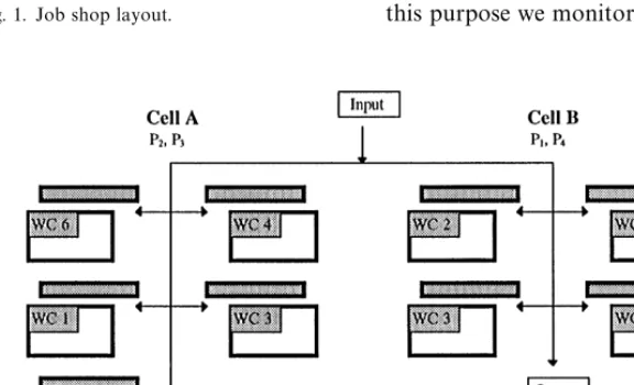
Shop layout: Job shop is a process layout and
involves a system resource organisation in isolated work centres in which all machines perform the same type of processing on parts to be produced (Fig. 1).
Fig. 2. Flexible cell shop layout. Fig. 1. Job shop layout.
Demandvariability:Demand variability has two
main components:
f Variability of inter-arrival time of lots to the
system;
f Balancing of product mix.
The "rst factor is modelled by means of the variation coe$cient of a log-normal distribution ranging from 0%, 40% and 100% of mean value. The second one is modelled by means of mix ratios selected so that system input is divided up among various families in accordance with a"xed
balanc-ing level (Fig. 3). In particular, the balancbalanc-ing is a function of P
1 load/P4 load ratio which ranges from 1 to 4 to 10 (Table 4).
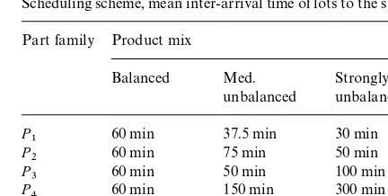
Considering a total system load of 20 parts per hour and a"xed lot size of 5 parts each, the sched-uling scheme is as shown in Table 5.
4.1. Simulation models
The three research questions are investigated with reference to the manufacturing system de-scribed in Section 3. Developing a full factorial experimental design, we consider 27 models de"ned by all possible combinations of experimental factor levels. These models were coded in a special soft-ware tool (WITNESS 7.0t). In de"ning simulation experiments three issues have been considered:
f the e!ect of bias deriving from starting
condi-tions, resulting in atypical system behaviour;
f observation time length of system events for each
simulation run;
f number of replications for each run (the
experi-ment sample size).
Fig. 3. Flow shop layout.
Table 4
Demand variability, levels of mix balancing Part family Product mix
Balanced Med.
unbalanced
Strongly unbalanced P
1 25% 40% 50%
P
2 25% 30% 30%
P
3 25% 20% 15%
P
4 25% 10% 5%
Mix ratio 1:1 4:1 10:1
Table 5
Scheduling scheme, mean inter-arrival time of lots to the system Part family Product mix
Balanced Med.
unbalanced
Strongly unbalanced P
1 60 min 37.5 min 30 min
P
2 60 min 75 min 50 min
P
3 60 min 50 min 100 min
P
4 60 min 150 min 300 min
Mix ratio 1:1 4:1 10:1
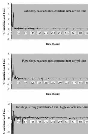
time percentage variation as signal for detecting bias e!ect deriving from starting conditions (use of alternative variables such as work in process, aver-age bu!er size etc. lead to the same results). Fig. 4 plots the trend of this variable over the"rst 30.000 running time units (minutes). As evident in this particular situation, plot #uctuations tend to fade away in about 210 hours. Clearly, at that moment, mean #ow time for manufactured parts becomes stable around its steady value.
Other plots show the same results for other experimental conditions, even if inter-arrival vari-ation provides persistent and larger #uctuations around the steady value, which is zero. In all cases, we can assume that transient state "nishes after
Fig. 4. Lead time percentage variation over time for di!erent models.
4.2. Performance measures:Dependent observed
variables
The dependent variables observed in steady state system simulation running have been selected ac-cording to literature indications [14] relatively to
most interesting manufacturing system perfor-mances and are abbreviated named as follows:
f LT: average lead time
f Buf. time: average time spent in bu!ers
f CV buf.: coe$cient of variation of bu!er time
spent in bu!ers
f Av. Util.: average work centres'utilisation f CV Util.: coe$cient of variation of work centres
utilisation
Besides, we add two other variables:
f Server: minimum number of servers in system f Volume: total system output
The"rst one is determined according to Eq. (1). It represents the total number of servers located to each work centre, i.e. the minimum resource neces-sary to respect the continuity bound and avoid system parts' accumulation, given an average expected utilisation. Hence, we consider this vari-able as a measure of performance, since its value re#ects the ability of the system to outperform the pre-assigned scheduled production, as a proper e$-ciency index. The second one quanti"es the number of parts shipped out from the system. Since we have imposed a resource sizing in order to avoid parts accumulation and observe steady state running, such a variable is not considered as a proper perfor-mance, because at any instant the steady continuity bound (System Input"System Output) is given. Such a condition imposes that total production volume will be always the same in each experimental condi-tion, not dependent on demand variability level or shop layout design (P
505, hourly total system input, was imposed equal to 20 parts). However, in this context, we consider this variable, since it will be very interesting to verify the veracity of consider-ations just exposed.
4.3. Other model assumptions
Utilised simulation models do not contemplate time consuming computation for material handling or inter-machine movements. Given the model assumptions, we suppose, in fact, that time shift due to parts movement does not impact system perfor-mances in a signi"cant manner. In reality the weight of move time on system performances (in particular on#ow time and queue related variables) can be very di!erent for di!erent shop layout
or-ganisations. In other words, part of the di!erence observed in lead time performance between job shop and#ow shop, can be explained in terms of move time of parts along manufacturing lines. But such an e!ect is not numerically relevant with respect to others, and in particular for those inter-ested in the aim of our research. Hence, we assume zero move time. Relevant components of time dependent variables are those due to set-up, ma-chine processes and in queue waiting.
5. Results analysis
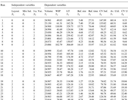
Experimental results of 27 simulation models, conducted to quantify the e!ect of independent variables on system performances, are shown in Table 6.
To answer research questions presented in Sec-tion 4,"rstly we proceed analysing results aiming to discover possible correlation between observed independent variables. So the correlation matrix for nine system performances was built in order to check the presence of a possible common trend. Such an analysis is shown in Table 7.
Choice of such a functional expression for e$-ciency index is justi"ed considering the positive e!ect of average system utilisation (Av. Util.) and the negative one of utilisation variation coe$cient (CV Util.) and total number of system servers (Ser-ver) on global performance. As expressed above, in fact, a manufacturing system is considered e$cient if the resource needed to process a given production volume is minimal (minimum Server), and if system work-load is well balanced between work centres (minimum CV Util, maximum Av. Util.). With ref-erence to the agility index it has been considered the negative e!ect of queue related performances (WIP, Buf. size, Buf. time), and of lead time. A manufacturing system is considered agile or lean if bu!ers content relains limited on time. This con-dition avoids system congestion, reduces produc-tion locking up and parts #ow times. Besides, in both cases, expressions involve constants for numerical normalisation of observed values.
Table 6
Mean values for observed dependent variables for each experimental model Run Independent variables Dependent variables
Layout Mix bal. I-a. Var. Volume WIP LT Buf. size Buf. time CV buf. Av. Util. CV Util. Server X
1 X2 X3 Y1 Y2 Y3 Y4 Y5 Y6 Y7 Y8 Y9
1 0 0 0 24.981 49.85 149.23 5.48 27.51 147.89 60.14 8.53 20
2 0 0 1 25.130 61.31 182.28 7.40 37.10 155.02 60.51 8.69 20
3 0 0 2 24.988 110.98 329.73 15.73 78.44 150.82 60.05 8.30 20
4 0 1 0 24.994 41.69 124.84 3.90 14.65 70.37 62.14 8.63 21
5 0 1 1 25.030 46.29 138.34 4.68 17.52 68.25 62.22 8.62 21
6 0 1 2 24.886 86.41 259.42 11.45 42.07 56.23 61.94 8.74 21
7 0 2 0 25.001 40.63 121.66 3.72 14.12 85.95 61.59 9.68 22
8 0 2 1 24.873 43.47 130.87 4.23 16.46 90.36 61.26 9.64 22
9 0 2 2 25.086 102.79 304.69 14.15 55.97 111.25 61.82 9.84 22
10 1 0 0 24.999 32.63 97.74 1.84 12.02 72.32 56.54 11.35 21
11 1 0 1 24.956 35.03 105.10 2.12 13.48 65.52 56.52 11.22 21
12 1 0 2 24.798 57.98 174.39 4.72 27.87 82.84 56.16 11.98 21
13 1 1 0 25.010 32.03 95.88 1.66 10.78 74.64 57.07 14.34 23
14 1 1 1 24.955 36.33 109.02 2.15 13.54 76.93 56.93 14.29 23
15 1 1 2 24.816 57.99 174.52 4.60 28.80 89.13 56.57 14.42 23
16 1 2 0 24.997 29.47 88.28 1.37 8.64 87.56 55.96 15.82 24
17 1 2 1 24.955 32.78 98.41 1.76 11.25 97.21 55.85 15.90 24
18 1 2 2 24.867 48.97 147.28 3.58 22.95 108.63 55.69 15.55 24
19 2 0 0 24.987 38.35 114.90 1.27 15.26 74.02 51.74 19.04 24
20 2 0 1 24.995 42.83 128.18 1.51 18.02 79.70 51.80 19.44 24
21 2 0 2 25.021 64.45 192.17 2.65 31.71 87.06 51.69 19.10 24
22 2 1 0 25.015 38.05 113.85 1.19 13.64 91.26 49.57 32.31 26
23 2 1 1 25.048 43.21 129.10 1.46 16.30 96.78 49.66 32.40 26
24 2 1 2 24.983 66.08 197.33 2.67 29.48 124.54 49.49 32.41 26
25 2 2 0 25.014 29.80 89.19 0.74 9.08 116.60 43.12 39.70 29
26 2 2 1 25.061 33.24 99.25 0.92 10.90 116.22 43.22 39.52 29
27 2 2 2 24.754 46.60 140.86 1.63 18.32 152.27 42.72 39.50 29
Table 7
Correlation matrix for observed dependent variables
Volume WIP LT Buf. Size Buf. time CV buf. Av. Util. CV Util. Server
Volume 1.000 0.002 !0.009 0.066 0.042 0.070 0.078 !0.010 !0.063
WIP 1.000 1.000 0.922 0.974 0.328 0.357 !0.307 !0.366
LT 1.000 0.922 0.973 0.326 0.357 !0.308 !0.366
Buf. size 1.000 0.925 0.271 0.582 !0.519 !0.556
Buf. time 1.000 0.424 0.360 !0.339 !0.412
CV buf. 1.000 !0.59 0.294 0.213
Av. Util. 1.000 20.958 20.927
CV Util. 1.000 0.961
Table 8
Components and numerical expressions for e$ciency and agility indexes
Cluster 2:Agility z WIP
z LT 106
WIP)LT)Buf.size)Buf.time z Buf. size
z Buf. time
are de"ned in a synthetic way through an e$ciency and agility index. Their numerical expression is underlined in Table 8.
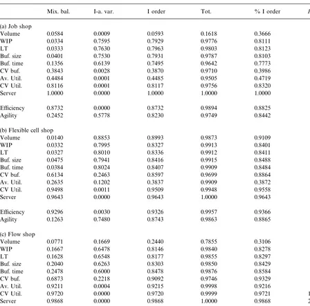
The statistical regression analysis allows to check the signi"cance of experimental factors with refer-ence to their in#urefer-ence on system performances, considering the hypotheses of a linear dependence. In Table 9 values of multiple correlation coe$cient
R2(columns 2}4) are listed for rating of"rst order e!ect for each di!erent shop layout con"guration. In column 5,R2value is presented for all the e!ects, up to third order, while in column 6 the ratio is relative to the percentage due to"rst order terms. Variance explained by experimental factors at"rst order level is rather high in cases highlighted in bold. In job shop and#ow shop cases volume seems not to be a!ected by experimental factors' vari-ations. Also the ANOVA test (F-value in column 7) strengthens such results. This observation is e!ec-tive for average utilisation too, for two of the three shop layouts.
The analysis clearly indicates that the impact of Inter-arrival time variation mainly regards the agil-ity performances (i.e. lead time, work in process, average bu!er size, average time spent in bu!er), while the impact of mix balancing variation mainly regards the e$ciency performances (i.e. number of servers in the system and variation coe$cient of resource utilisation).
Through aStudent T-test, statistical results analy-sis allowed to highlight the presence of meaningful di!erences in performance mean values, observed
in groups corresponding to the experimental factor level combinations. Preliminary F-test was performed to test the homogeneity of means for di!erent groups examined, by means of sample data analysis. In Table 10 StudentT-test data are listed. Almost all di!erences observed by varying shop layout level are signi"cant at an a level of about 0.05 (bold values). We cannot have the same statement for mix balancing factor, while relatively to inter-arrival time variation we observe a signi"-cant di!erence in system behaviour (particularly for queue related performances), for groups of 0 and 2 levels. That is, only for a remarkable increase in inter-arrival time variability (variation coe$cient ranging from 0% to 100%), a real worsening of system agility can be stated.
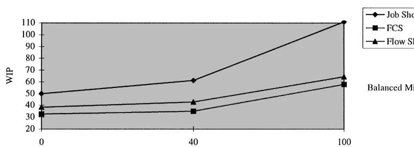
In curves shown in Figs. 5}8 the e!ects whose statistics are signi"cant, are plotted with reference to di!erent experimental conditions.
Queue related performances deteriorate against inter-arrival time variability increase (Fig. 5). Job shop layout shows the worst levels, while#exible cell shop the best ones. The plotted trend is the same for the lead time variable (Fig. 6), but in this case the unbalancing#attens curves of#exible cell shop and#ow shop layouts.
Fig. 7 shows that, apart from system input variability, the choice of a shop layout with dedi-cated resources involves a decrease in system e$-ciency, in terms of average work centres utilisation. Besides, the curve has a rather similar trend for di!erent mix balancing conditions (plots not pre-sented here). The only experimental factor having a strong e!ect on such a variable is hence the shop layout design.
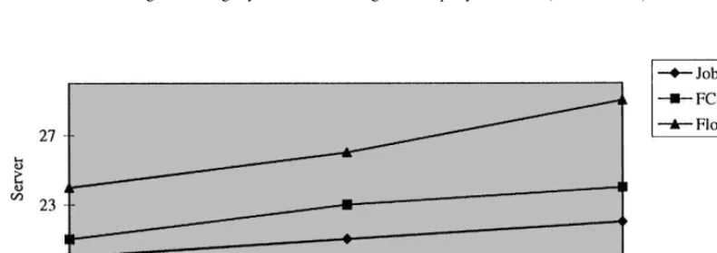
Instead, in terms of mix balancing variability, the only e!ect supported by statistical indexes is rela-tive to the dependent variable named server. Mix unbalancing implies an increase of resource needed in work centres (Fig. 8). In fact it involves an in-crease in the presence of parts characterised by longer sequences and longer processing times. Hence, the most evident e!ect is the increase of system load, with consequent need for additional servers, as established in Eq. (1).
Table 9
Multiple regression coe$cient (R2) and test-Ffor each observed variable
Mix. bal. I-a. var. I order Tot. % I order F-value
(a) Job shop
Volume 0.0584 0.0009 0.0593 0.1618 0.3666 0.1892!
WIP 0.0334 0.7595 0.7929 0.9776 0.8111 11.4860
LT 0.0333 0.7630 0.7963 0.9803 0.8123 11.729
Buf. size 0.0401 0.7530 0.7931 0.9787 0.8103 11.4983
Buf. time 0.1356 0.6139 0.7495 0.9642 0.7773 8.9745
CV buf. 0.3843 0.0028 0.3870 0.9710 0.3986 1.8942!
Av. Util. 0.4484 0.0001 0.4485 0.9505 0.4719 2.4398!
CV Util. 0.8116 0.0001 0.8117 0.9756 0.8320 12.9283
Server 1.0000 0.0000 1.0000 1.0000 1.0000 d
E$ciency 0.8732 0.0000 0.8732 0.9894 0.8825 20.6522
Agility 0.2452 0.5778 0.8230 0.9749 0.8442 13.9473
(b) Flexible cell shop
Volume 0.0140 0.8853 0.8993 0.9873 0.9109 26.7810
WIP 0.0332 0.7995 0.8327 0.9913 0.8401 14.9329
LT 0.0327 0.8010 0.8336 0.9912 0.8411 15.0342
Buf. size 0.0475 0.7941 0.8416 0.9915 0.8488 15.9341
Buf. time 0.0384 0.8024 0.8407 0.9909 0.8484 15.8362
CV buf. 0.6134 0.2463 0.8597 0.9699 0.8864 18.3870
Av. Util. 0.2635 0.1202 0.3837 0.9909 0.3872 1.8677!
CV Util. 0.9498 0.0011 0.9509 0.9948 0.9558 58.1273
Server 0.9643 0.0000 0.9643 1.0000 0.9643 81.0000
E$ciency 0.9296 0.0030 0.9326 0.9957 0.9366 41.5118
Agility 0.1263 0.7480 0.8743 0.9863 0.8865 20.8710
(c) Flow shop
Volume 0.0771 0.1669 0.2440 0.7855 0.3106 0.9680!
WIP 0.1667 0.6478 0.8146 0.9840 0.8278 13.1791
LT 0.1628 0.6548 0.8177 0.9855 0.8297 13.4544
Buf. size 0.2040 0.6263 0.8303 0.9850 0.8429 14.6768
Buf. time 0.2478 0.6000 0.8478 0.9876 0.8584 16.7052
CV buf. 0.6873 0.2218 0.9092 0.9746 0.9329 30.0310
Av. Util. 0.9211 0.0004 0.9215 0.9998 0.9216 35.1925
CV Util. 0.9720 0.0000 0.9720 0.9999 0.9721 104.0524
Server 0.9868 0.0000 0.9868 1.0000 0.9868 225.0000
E$ciency 0.9422 0.0000 0.9422 0.9998 0.9425 48.9354
Agility 0.3400 0.3673 0.7073 0.9594 0.7372 7.2481
!Not signi"cant.
shown for di!erent combinations of experimental factors.
Histograms built on such data are plotted in Figs. 9}11. With reference to research question 1 expressed in Section 4, it can be possible to
Table 10
Test-tfor mean values di!erence of observed performance groups
Level comparison Shop layout Mix balancing I-a variability
0}1 0}2 1}2 0}1 0}2 1}2 0}1 0}2 1}2
Volume 0.093 0.804 0.170 0.734 0.555 0.746 0.987 0.047 0.067
WIP 0.034 0.074 0.454 0.618 0.401 0.645 0.227 0.002 0.005
LT 0.034 0.074 0.469 0.627 0.401 0.640 0.225 0.002 0.004
Buf. size 0.010 0.004 0.041 0.602 0.578 0.917 0.535 0.042 0.072
Buf. time 0.053 0.073 0.690 0.301 0.234 0.729 0.336 0.006 0.014
CV buf. 0.171 0.987 0.047 0.211 0.699 0.023 0.826 0.265 0.372
Av. Util. 0.000 0.000 0.000 0.982 0.395 0.422 0.997 0.948 0.945
CV Util. 0.000 0.000 0.000 0.196 0.105 0.586 0.995 0.993 0.998
Server 0.006 0.000 0.001 0.096 0.014 0.208 1.000 1.000 1.000
E$ciency 0.000 0.000 0.000 0.443 0.152 0.553 0.993 0.976 0.983
Agility 0.021 0.055 0.614 0.684 0.122 0.164 0.242 0.025 0.030
Fig. 5. Average work in process against inter-arrival time CV (balanced mix).
is evident that a shop with dedicated lines has the fastest queue dynamics, making easier the execu-tion of dispatched orders for parts producexecu-tion. Line dedication makes possible to avoid system over-load so that it maintains a low steady level of agility over time. On the contrary, job shop proves to be more e$cient, since production#ows are designed and managed stressing the importance of load bal-ancing among system work centres. This condition imposes the rationalisation of system resources. Consequently, it implies a better work centres' average utilisation, a reduction in bottlenecks' criti-cality and a lower number of servers needed
to execute orders assigned for production of dispatched parts.
Fig. 6. Average lead time against inter-arrival time CV (strongly unbalanced mix).
Fig. 7. Average system utilisation against shop layout choice (balanced mix).
Table 11
Mean values for e$ciency and agility indexes
E$ciency Agility
Job 32.7818 1.4459
Layout FCS 18.4445 11.3107
Flow 6.9569 14.8392
0% 19.4673 17.2102
I-a variability 40% 19.4190 9.2331
100% 19.2969 1.1525
High 23.3302 5.0043
Mix balancing Medium 19.0858 6.1863
Low 15.7671 16.4052
Fig. 9. Macro performances against shop layout design.
Fig. 10. Macro performances against mix balancing.
Fig. 11. Macro performances against lots inter-arrival time variability.
both signi"cant and generalisable, so that it is not possible to state anything about the impact of such factors on system performances. With regard to lots inter-arrival time variability, data in Table 11 show that system e$ciency does not depend in any way on this factor. On the contrary, the impact on system agility is very heavy because of the e!ect
driven on work centres bu!ers "lling dynamics. While lots inter-arrival time increases, the #uctu-ation range of queues content increases heavily and irregularly over time. Such an e!ect implies a signif-icant worsening of system agility mean value, as plotted in Fig. 11. So, aiming to answer research questions 2 and 3, it can be stated that demand variability has a strong e!ect only on system agility and not on e$ciency performances. Besides, this e!ect is due to lots inter-arrival time variability and not to mix balancing.
6. Conclusions
In this paper three alternative manufacturing layouts (job shop,#exible cell shop,#ow shop) are compared aiming to test their robustness with respect to system input variability, modelled through the variation coe$cient of lots' inter-arri-val time to the system and unbalancing of product mix. Results obtained by means of simulation ex-periments show that trade-o!between set-up sav-ing and routsav-ing#exibility has a well evident impact on system macro performances: agility and e$cien-cy. Set-up saving allows to reduce in-queue waiting time, routing#exibility allows to minimise process resources assigned to the manufacture system. So alternative layout con"gurations have opposite be-haviour. Job shop process layout involves a system resource organisation which provides best e$cien-cy performances (average utilisation, utilisation balancing, number of servers needed,2), since the
nature of resources allows maximum set-up saving but, at the same time, provides routing in#exibility. So having the best queue related performances (work in process, average bu!er size, average bu!er time, lead time,2) it is necessary to revert to
e$-ciency. Obviously, hybrid forms should provide intermediate performance. Flexible cell shop layout ensures an intermediate level of set-up saving and an intermediate level of routing #exibility, i.e. an intermediate level of e$ciency and agility.
Considering di!erent demand variability condi-tions, in terms of inter-arrival time variation and mix balancing, the experimental analysis proved that the larger e!ect on system performances is due to the"rst factor, not to the second one. However, this e!ect is limited to agility performances (queue and time related performances). System e$ciency seems not to depend on demand variability.
Such results indicate that manufacturing layout choice depends on the particular performance con-sidered critical by the decision maker. There does not exist a layout that overcomes others in an absolute way. Each one is characterised by a proper level of routing#exibility and set-up saving.
With respect to literature indications, this paper returns consistency to the hypotheses of cellular manufacturing layout choice, which guarantees in-termediate level of system e$ciency and agility.
Empirical evidence shows that layout alternative to job shop or, in general, functional forms, almost always brought a signi"cant improvement in over-all system performance. The need to solve this contradiction between theoretical models and em-pirical research, points out that in comparative theoretical studies (like the presented one), some critical factors are not considered, such as labour, labour}machine interaction, run time (and not only set-up) reduction, inter-cell movement, not instan-taneous movement, and so on.
So, this study would not mind a methodological contribution to the choice of the best manufactur-ing layout, due to the data-dependent nature of system performance, but it proposes some clarify-ing elements for the decision makclarify-ing process which companies apply when they decide to implement or convert their manufacturing layout.
Results obtained in this research have to be checked for a more complex manufacturing system.
Authors are performing a sensitivity analysis to test signi"cance of part-machine matrix size on present-ed research questions. It would be interesting also to remove the hypotheses of zero move time and quantify the e!ect of other demand related vari-ables, such priority assignment for families schedul-ing, rules for bu!er scheduling and so on.
References
[1] J.S. Noble, J.M.A. Tanchoco, Design justi"cation of manu-facturing systems, The International Journal of Flexible Manufacturing System 5 (1993) 5}25.
[2] J.S. Morris, R.J. Tersine, A simulation analysis of factors in#uencing the attractiveness of group technology cellular layouts, Management Science 36 (12) (1990) 1567}1578. [3] B.J. Jensen, M.K. Malhotra, P.R. Philipoom, Machine
dedication and process#exibility in a group technology environment, Journal of Operations Management 14 (1996) 19}39.
[4] N.C. Suresh, Partitioning work centers for group techno-logy: Analytical extension and shop-level simulation investigation, Decision Sciences 23 (2) (1992) 267}290. [5] N.C. Suresh, Partitioning work centers for group
techno-logy: Insights from an analytical model, Decision Sciences 22 (1991) 772}791.
[6] N.C. Suresh, J.R. Meredith, Coping with the loss of pool-ing synergy in cellular manufacturpool-ing systems, Manage-ment Sciences 40 (4) (1994) 466}483.
[7] B.B. Flynn, F.R. Jacobs, An experimental comparison of cellular (group technology) layout with process layout, Decision Sciences 18 (1987) 562}581.
[8] C.L. Ang, P.C. Willey, A comparative study of the perfor-mance of pure and hybrid group technology manufactur-ing systems usmanufactur-ing computer simulation techniques, The International Journal of Production Research 22 (1984) 193}233.
[9] R. Leonard, K. Rathmill, The group technology myths, Management Today January (1977) 66}69.
[10] C.A. D'Angelo, M. Gastaldi, N. Levialdi, Dynamic analy-sis of a#exible manufacturing system: A real case applica-tion, Computer Integrated Manufacturing Systems 9 (2) (1995) 101}110.
[11] C.A. D'Angelo, M. Gastaldi, N. Levialdi, Performance analysis of a#exible manufacturing system: A statistical approach, International Journal of Production Economics 56/57 (1998) 47}59.
[12] R.G. Askin, C.R. Standridge, Modeling and Analysis of Manufacturing Systems, Wiley, New York, 1993. [13] G.S. Fishman, Estimating sample size in computer
simula-tion experiments, Management Science 18 (1971) 21}38. [14] A. D'Angelo, M. Gastaldi, N. Levialdi, Optimizing#ows