CONJECTURING PRODUCTION, IMPORTS AND CONSUMPTION OF HORTICULTURE IN INDONESIA IN 2050: A GAMS SIMULATION THROUGH
CHANGES IN YIELDS INDUCED BY CLIMATE CHANGE
Pendugaan Produksi, Impor, dan Konsumsi Hortikultura
di Indonesia Tahun 2050: Simulasi Gams Melalui Perubahan Produktivitas Karena Pengaruh Perubahan Iklim
Budiman Hutabarat1, Adi Setiyanto1, Reni Kustiari1, and Timothy B. Sulser2
1Indonesian Center for Agriculture Socio Economic and Policy Studies (ICASEPS) Jl. A. Yani No. 70 Bogor 16161, Jawa Barat, Indonesia
2
International Food Policy Research Institute (IFPRI) Washington, DC, USA
Naskah masuk : 21 Maret 2012 Naskah diterima : 2 April 2012
ABSTRACT
Petunjuk perubahan iklim yang cepat saat ini telah diamati dan dibukukan secara meluas. Semua perubahan ini secara pasti akan menyebabkan kemerosotan jumlah dan mutu lahan, air, dan iklim mikro di tempat di pertumbuhan tanaman hortikultura. Selanjutnya, dapat diprakirakan produktivitas lahan dan hortikultura akan menurun. Makalah ini bertujuan untuk mengkaji pengaruh yang dipicu perubahan ini pada produksi, impor, dan konsumsi produk hortikultura. Penelitian ini menggunakan pendekatan model keseimbangan parsial pasar-jamak dalam kerangka simulasi. Semua hasil-hasil simulasi IFPRI memprakirakan bahwa produktivitas kelompok buah (pisang dan jeruk) dan sayuran (cabai dan bawang merah) meningkat dibandingkan keadaan baseline. Demikian pula, apabila perbandingan dilakukan terhadap hasil skenario tidak terjadi perubahan iklim (NoCC), kesimpulan yang berbeda akan diperoleh. Pada tahun 2050, model ini memberikan petunjuk yang berlainan dengan hasil literatur dan hipotesis yang menyatakan bahwa produksi, impor, dan konsumsi terhadap hortikultura akan menurun. Sebaliknya model mengantisipasi bahwa produksi pisang, jeruk, cabai, dan bawang akan meningkat di perdesaan Jawa dan Luar-Jawa. Namun, hasil-hasil ini harus ditafsirkan secara hati-hati berhubung kesulitan penarikan kesimpulan atas pengaruh perubahan iklim terhadap komoditas hortikultura yang berlaku secara umum, karena komoditas hortikultura jumlahnya beribu-ribu dengan sifat masing-masing yang khas. Untuk itu kajian dan penelitian yang intensif dan menyeluruh sangat diperlukan karena perubahan iklim bukanlah fenomena jangka pendek seumur tanaman, tetapi bersifat jangka panjang. Dalam kaitannya dengan indikator perdagangan, simulasi memberikan hasil yang sama bahwa impor pisang, jeruk, cabai, dan bawang akan meningkat, tetapi impor kedua komoditas terakhir tidak besar. Skenario CSIRO_A1b, CSIRO_B1, dan MIROC_A1b memproyeksikan konsumsi nasional agregat pisang, jeruk, cabai, dan bawang akan menurun dengan perubahan iklim, tetapi meningkat menurut Skenario MIROC_B1 . Namun, terlihat ada perbedaan konsumsi komoditas-komoditas ini antarwilayah. Konsumsi rumah tangga di Jawa menurun pada 2050, penurunan ini akan sangat terasa pada keluarga miskin di Jawa. Sementara itu, konsumsi semua kelompok rumah tangga di Luar Jawa meningkat, kecuali menurut Skenario MIROC_A1b dan Skenario CSIRO_B1, di mana konsumsi keluarga miskin di Luar Jawa menurun. Makalah menyarankan agar penelitian perakitan kultivar yang dapat menyesuaikan diri dan tahan kekeringan dan juga teknik-teknik penghematan air yang sesuai untuk tanaman hortikultura atau penggunaan air secara efisien perlu ditingkatkan. Teknologi-teknologi semacam ini sangat dibutuhkan saat ini. Cara-cara penyebarluasan atau pengkomunikasian kultivar-kultivar dan teknologi-teknologi di atas ke pihak petani kecil juga perlu digali lagi agar mereka dapat memanfaatkannya.
ABSTRACT
Indication of Earth’s changing climate with rapid pace currently present time has been observed and extensively documented. All these changes will undoubtedly lead to deterioration in quantity and quality of land, water, and micro-climate where the horticultural crops are grown. Subsequently, it can be anticipated that land and horticultural productivity will be depreciated. The purpose of this paper is to investigate the impact of this induced change in these horticultural crops on the production, imports, and consumption of these crops. This study adapts a multimarket model of partial equilibrium analysis to a simulation framework. All scenarios adopted by the IFPRI study predict that the yields of fruit crop group (bananas and oranges) and vegetables (chilies and shallots) would increase compared to the baseline scenarios. But by making comparison to no climate change (NoCC) scenario after simulating it from the baseline, mixed conclusions are obtained. For 2050, the model anticipates increases in the production of bananas, oranges, shallot, and chilies by rural households in Java and Off-Java. These findings have to be interpreted cautiously, because it is extremely difficult to make a general conclusion about the impact of climate change on horticulture for the fact that horticulture consists of thousands of crops, of which each of them has unique characteristics. More intensive and comprehensive studies are still required because climate change is not a short-term phenomenon of crop-cycle. In regard to net trade indicators, this study foresees that bananas, oranges, chilies and onions imports would grow but the rate of growth of chilies’ and onions’ imports are not significant. National consumption of bananas, oranges, chilies and shallot are projected to fall under Scenarios CSIRO_B1 and MIROC_A1b but it increases under Scenario MIROC_B1. However, there would be disparities in consumption of bananas, oranges, chilies and shallot among regions. Java households will experience decreases in consumption in 2050, whereas Java–poor households would suffer the most. On the other hand almost all types of Off-Java households will enjoy a positive rate of consumption changes, with the exception being the results of Scenario MIROC_A1b and Scenario CSIRO_B1 for Off-Java–poor households, which indicate a decrease in consumption. This paper recommends that more researches on assembling cultivars adaptable or tolerable to drought as well as appropriate technologies to conserve water for horticultural crops and to use the limited amount of water efficiently are in high demand today. Best means to disseminate or communicate these cultivars and technologies to smallholding horticultural-farmers ought to be explored.
Key words: horticulture, climate change, scenario, small farmers
INTRODUCTION
Emissions Trading Scheme (ETS). It is true that concentrations of CO2 in atmosphere would accelerate and could advance productivities of most horticultural crops1, but the extent of this benefit is unknown and merits investigation. All these changes will undoubtedly lead to deterioration in quantity and quality of land, water, and micro-climate where the horticultural crops are grown. Subsequently, it can be anticipated that land and horticultural productivity will be depreciated.
In Indonesia the consequence of climate change in agriculture has not been addressed proportionally, although this sector remains to be a very important agent of development that is expected to boost production and improve rural population’s well-being. For horticulture, a component in agriculture, the interest to design its architectural development in 10 to 20 years in the future is bleak at best. This sub-sector, represented by four sets of crop, namely fruits, vegetables, floriculture, and medicinal crops was able to create a positive growth in export values at about 22 percent in 2007 to 2011 period (Table 1), which predominantly comes from fruits and medicinal crop exports. Notwithstanding, Indonesia’s horticultural import also goes up at almost the same rate as that of the export values, which happens greatly through floriculture and vegetable crop imports .
The table shows that the average growth of import values is lower than that or export values, but the gaps between the value of exports and that of imports of fruits and vegetables are widening, which suggests that Indonesia imports more than it exports on these two commodities. Moreover, despite floriculture and medicinal crop exports grow at high rates, their bases are far behind those of fruits and vegetables, only about 2 to 3 percent of total export values of horticultural crops. It means that even though these two crops may have prospects to be developed for export market, but at present they remain unable to substitute for fruits and vegetables in terms of collecting foreign exchanges. Given that situation, it is envisaged that under climate change the yield, production, and net export of Indonesia’s horticulture will be impaired in the future. Unfortunately, in the literature, empirical research on the impact of climate change on horticulture is hardly available. From its extensive research and simulation work using IMPACT model, the International Food Policy Research Institute/IFPRI has produced some figures about the impact of climate change on the yields of many agricultural crops, including horticulture throughout regions of the world. The purpose of this paper is to investigate the impact of this induced change in these horticultural crops on the production, imports, and consumption of horticultural crops.
The paper is arranged in such a way as follows: section 2 reviews some literature that provides evidence of climate change and its impact on horticulture in selected regions and in Indonesia. Section 3 explains briefly about the model used to estimate the climate change impact in agriculture, followed by section 4 containing the results of estimation and discussion. The final section summarizes all the results to come up with conclusion and policy recommendation.
CLIMATE CHANGE EVIDENCE
Based on scientific measurement on some indicators such as sea level, global temperature, oceans’ temperature and acidity, ice sheets, Arctic sea ice, glacial retreat NASA (2012) reiterates that climate change has been overwhelming. On the on-line journal of Global Climate Change: Vital Signs of the Planet, NASA issues some evidences of these claims: (i) sea level rise; in the last century, global sea level rose about 17 centimeters, but in the last decade, the rate is nearly double that of the last
century (Church and White (2006) in NASA ( on-line 2012); (ii) global temperature rise; All three major global surface temperature reconstructions (NCDC line 2012, CRU on-line 2012, GISS on-on-line 2012) show that Earth has warmed since 1880. Most of this warming has occurred since the 1970s, with the 20 warmest years having occurred since 1981 and with all 10 of the warmest years occurring in the past 12 years (Peterson et.al. (2009) in NASA (on-line 2012)). Even though the 2000s witnessed a solar output decline resulting in an unusually deep solar minimum in 2007-2009, surface temperatures continue to increase (Allison et.al. (2009) in NASA (on-line 2012)); warming oceans, the oceans have absorbed much of this increased heat, with the top 700 meters (about 2,300 feet) of ocean showing warming of 0.302 degrees Fahrenheit since 1969 (Levitus, et al. (2009) in NASA (on-line 2012)); declining Arctic sea ice, both the extent and thickness of Arctic sea ice has declined rapidly over the last several decades ( Polyak, et.al. (2009) and Kwok and Rothrock (2009) in NASA (on-line 2012)); glacial retreat, Glaciers are retreating almost everywhere around the world — including in the Alps, Himalayas, Andes, Rockies, Alaska and Africa (NSIDC on-line 2012 in NASA (on-line 2012)) and WGMS on-line 2012 in NASA (on-line 2012)); ocean acidification, Since the beginning of the Industrial Revolution, the acidity of surface ocean waters has increased by about 30 percent (PMEL (on-line 2012a) and PMEL (on-line 2012b) in NASA (on-line 2012)). This increase is the result of humans emitting more carbon dioxide into the atmosphere and hence more being absorbed into the oceans. The amount of carbon dioxide absorbed by the upper layer of the oceans is increasing by about 2 billion tons per year (Sabine et.al. (2004) in NASA (on-line 2012)) and The Copenhagen Diagnosis (on-line 2012) in NASA (on-line 2012)).
Bringing it closer to home PEACE (2007) has documented some impacts of climate anomalies in Indonesia, specifically through El Nino and La Nino events, although the evidence of intense and more frequent El Nino and La Nina events have not been attested to cause or to be caused by climate change. Annual mean temperature in Indonesia has been observed as increasing by around 0.3 degrees Celsius (o C) since 1990 and has occurred in all seasons of the year, relatively consistent if not slightly lower than the expectation of the warming trend due to climate change (Hulme and Sheard (1999) in Case et al. (No date)). Annual precipitation overall has decreased by two to three percent across all of Indonesia over the last century. However, there is significant spatial variability, a decline in annual precipitation in the southern regions of Indonesia (e.g., Java, Lampung, South Sumatra, South Sulawesi, and Nusa Tenggara) but an increase in rainfall in the northern regions of Indonesia (e.g., most of Kalimantan, North Sulawesi) (Boer and Faqih, 2004).
The seasonality of precipitation (wet and dry seasons) has also shifted; in the southern region of Indonesia the wet season rainfall has increased while the dry season rainfall has decreased, whereas in the northern region of Indonesia the opposite pattern was observed (Boer and Faqih, 2004). It should be noted that precipitation in Indonesia (and many parts of the world) is strongly influenced by El Niño/ Southern Oscillation (ENSO) events and that some researchers suggest that there will be more frequent and perhaps intense ENSO events in the future because of the warming global climate (Tsonis et al., 2005). Because Indonesia typically experiences droughts during El Niño events (the warm phase of ENSO) and excessive rain during La Niña events (cool phase of ENSO), this global pattern will have regional impacts.
in fair to poor condition (Johns Hopkins University 2003 in PEACE (2007)). A survey in the Bali Barat National Park found that a majority of coral reefs were in poor condition. More than half of the degradation was due to coral bleaching. In the late 1990s, El Nino and La Nina events were also held responsible for outbreaks of malaria, dengue and plague.
Table 1. Export and Import Values of Indonesia’s Horticulture, 2007-2011 (US$ million)
Export values (US$ million)
a The export value of medicinal crops are excluded to warrant for comparison.
METHODOLOGY
Modeling the Impact of Climate Change for Indonesia
This study employs an approach that adapts a multimarket model of partial equilibrium analysis following Sayaka et al. (2007a, 2007b). Incidentally, Sayaka et al. derived their models from those formulated by Stifel and Randrianarisoa (2004) and Stifel (2004), which, in turn, are a modification of the generic model on agricultural policy reform generated by Lundberg and Rich in the World Bank report 2002 (cited in Stifel 2004). In this study, we extended the model by adding more commodity coverage and relaxing the assumptions that Sayaka et al. (2007a, 2007b) made that some products are not tradable or are only domestically produced ) to reflect the condition of Indonesia’s economy in the late 2000s.
Description of the Model
A general description of the product and household categories used in the model are as follows:2
• Product categories consist of the main agricultural outputs and inputs that drive Indonesia’s agriculture sector, such as (1) crop products—rice, maize, soybeans, cassava, bananas, peanuts, sweet potatoes, oranges, onions, chilies, potatoes, palm oil, coconut oil, cocoa, coffee, sugar, and wheat; (2) animal products—meat, eggs, and milk; and (3) agricultural inputs—urea fertilizer, phosphorus and potassium fertilizer, and maize for animal feed.
• Household groups are made up of two main groups: (1) urban households, comprising urban–rich, urban–middle-income, and urban–poor, and (2) rural households, comprising Java–rich, Java–middle-income, Java–poor, Off-Java–rich, Off-Java–middle-income, and Off-Java–poor.
Structure of the Model
Following Lundberg and Rich’s (2002) generic model, the model applied here contains six blocks of equations in the multimarket model: prices, supply, input demand, and product consumption, income, and equilibrium conditions. Theprice blockdefines the relationship between producer prices and consumer prices in the domestic economy based on the degree of transactions costs. For tradable goods, domestic prices are related to world prices, whereas prices of non-traded goods are determined by supply-and-demand conditions. The supply block represents the domestic production of food crops, livestock, and nonagricultural production. The input demand block describes the household demands for agricultural inputs. The consumption block shows household demand for food and nonfood consumption items. Theincome blockdescribes household income as the sum of income derived from agricultural production and exogenous nonagricultural income. The equilibrium conditions block contains equations that relate domestic supply and net import to demand for each of the 23 products.
Each block of equations is written in mathematical formulation as follows:
2
Price Block
Producer prices (PP) for each household group (H) are lower than consumer prices (PC). The band between these prices is determined exogenously by commodity-specific (c) domestic marketing margins (MARGc) as a proxy for transportation costs:
PPc,h = PCc,h/(1 +MARGc). (1)
For all of these (tradable) products, however, prices are determined exogenously by fixed world prices, with net imports (imports less exports) clearing the domestic market (that is, filling the gap between domestic demand and supply at the fixed prices). As a consequence, we must differentiate among world, border, and consumer prices and establish their relationships. The border prices of importable products (PM) are linked to the world price (PW) by the exchange rate (er), import tariffs (tm), and the international
marketing margin (RMARG):
PMc = PWc* [er* (1 +RMARGc)] * (1 +tm). (2)
Consumer prices for importable items (PMC) are related to the border price
(equivalent to consumer prices faces by the urban rich (urbrich)) by the commodity-specific border-to-market marketing margin (IMARG):
PMc = PCurbrich,c/(1 +IMARGc). (3)
Rural consumer prices (rh) differ from urban consumer prices by an internal marketing margin (INTMARGc), which reflects transportation and marketing costs which
can differ by commodity:
PCrh,c = PCurbrich,c/(1 +INTMARGc,rh). (4)
Finally, price indices for each household group (PINDEXh) are included to reflect
changes in prices from the base case (PC0) weighted (PCWT) by their shares of consumption:
PINDEXh = Σ (PCWTh,c* 0.4) *PCh,c/PC0h,c + 0.6. (5)
Supply Block
Household supply of food crops (f)—fine grains, coarse grains, roots and tubers, cash crops, and other food products—is determined by (1) the total quantity of land available to each household, (2) the share of that land allocated to specific crops, and (3) the associated yield for the crops. We begin with an initial total amount of land under cultivation (AREA0). Each household group can reallocate land among the food crops (except for estate crops of palm oil, coconut oil, cocoa, and coffee) to maximize profits. Thus, the share of land owned by household group allocated to the cultivation of food crop (SHrh,f) is determined by the prices of all food crops:
log(SHrh,f) = αsrh,f + Σβsh,i,I *log(PPrh,f). (6)
The yields of food crops for household groups (YLDh,f) are represented in
log-linear form as a function of output prices and input prices (in), proxying for conditional input demand and climate change impact on productivity (RDE):
log(YLDrh,f) =αyrh,f +βyrh,f *log(PPrh,f) + Σγh,f,I *log(PCrh,in) * log(PCrh,in) +
δf*log(RDEf) + , (7)
where f represents rice, maize, soybeans, cassava, bananas, peanuts, sweet potatoes, oranges, onions, chilies, potatoes, palm oil, coconut oil, cocoa, coffee, and sugar and the coefficients represent price elasticities. Total household supply to the market is then determined as the product of the initial area of cultivated land, the share of land devoted to the crop, and the yield. Further, this amount is adjusted for losses, for the use of the output for seed (loss), and for any related conversion factors (CONV), such as converting paddy to rice:
HSCRrh,f =AREA0 *SHARE0rh,f *YLDrh,f *CCFactorf * (1 - PERTE0f )* CONVf. (8)
The total supply (SCR) of each of the sixteen food crops is the sum of household supply (HSCR):
SCRf = ΣHSCRrh,f. (9)
Household supply of livestock commodity (l) - meat, eggs, and milk, (HSLVrh) is
represented as functions of their own producer prices. As with food crops, the total of the market supply of livestock (SLV) is equal to the sums of the various household supplies:
log(HSLVrh,l) = αlrh + βlrh,l,l *log(PPrh,l) + Σγrh,af,I *log(PCrh,af), (10)
SLV(L) = ΣHSLVi,l (11)
whereaf is input of livestock production, that is, maize for animal.
Input Demand Block
Each household group’s demand for agricultural input (HDINrh,in) is a function of
the input’s price and the prices of the food crops for which the inputs are used. The demand function is in the form
log(HDINrh,in) =αfrh,in + Σβrh,f,i *log(PPrh,f) + γfrh,in *log(PCrh,in) * log(PCrh,in), (12)
where the subscript in refers to animal feed, urea fertilizer, phosphorus, and potassium fertilizer. Total demand for the inputs is given by
DINin = ΣHDINi. (13)
Consumption Block
functions of their own producer, (HC) by the household groups in urban and rural locations is written as
log(HCh,i) =αhh,i + Σβhh,i,j *log(PCh,j) + γhh,i *log(YHh), (14)
where i refers to commodities purchased by households and YH is household income (defined later in this section), and PC is consumer prices. Total demand for each commodity is the sum of the household demands:
CONSi = ΣHCi,h. (15)
Equilibrium Conditions
Economic equilibrium requires that each product market is clear. For each food crop, this means that the total quantity supplied (sum of domestic supply and net imports) is equal to the total quantity demanded, that is the sum of demand by households (CONSf), animal feed (CONANIMf), other uses (CONSOTHR0f), private stocks
(PRSTKS0f), and government stocks (GOSTKS0f):
SCRf +NIMf =CONSf +CONANIMf +CONSOTHR0f +PRSTKS0f +
GOSTKS0f (18)
for rice, maize, soybeans, cassava, bananas, peanut, sweet-potato, oranges, onion, chili, potato, palm oil, coconut oil, cocoa, coffee, and sugar;
NIMnp =CONSnp +CONANIMnp +CONSOTHR0np +PRSTKS0np +
GOSTKS0np (19)
for wheat;
SINin = DIN0in (20)
for urea, phosphorus, and potassium fertilizer; and
SLVl +NIMl =CONSl +PRSTKS0l +GOSTKS0l (21)
for livestock products: meat, eggs, and milk.
Types and Sources of Data
To empirically apply this type of structural model, it is necessary to first calibrate the model to the data. In line with this paper’s objective to examine the impact of climate change on Indonesia’s agriculture, the model is calibrated to a baseline solution that describes Indonesia’s agriculture in 2008. Three types of data are required.
2. Prices: Initial consumer, producer, user, and border prices must be defined for each commodity; these prices then define the marketing margins. Producer and consumer prices are taken from BPS, MoA, the Ministry of Trade/MoT, Badan Urusan Logistic/BULOG or Logistic Agency, or other sources.
3. Behavioral parameters: These are the demand and supply elasticities (β’s and γ’s in the equations). Most are either collated from research papers of undergraduate or graduate students in various universities in Indonesia or estimated from survey data; a few others are best guesses in the absence of reliable data. An overview of the elasticities is as follows:
o Land-share elasticities (equation (6)): The own-price elasticities range from 0.186
(for onions) to 0.298 (for palm oil). Nearly all cross-price elasticities with respect to other crops are negative, spanning from –0.324 to –0.001. The one exception, in which the cross-price elasticity is positive, is coconut oil production with respect to the price of bananas, which is 0.044.
o Crop-yield elasticities (equation (7)): The own-price elasticities of all food crops
extend from 0.229 to 0.337. Crop-yield elasticity with respect to urea price range from –0.033 to –0.083, and to phosphorus and potassium fertilizer price is between –0.074 to –0.030.
o Livestock product supply elasticity (equation (10)): The own-price elasticities are
all positive (between 0.189 and 0.460). The cross-price elasticities are also all positive (from 0.021 to 0.651). The price elasticities of livestock supply with respect to the price of animal feed are all negative (from –1.750 to –0.445).
o Input-demand elasticities (equation (12)): The own-price elasticity of demand for
urea fertilizer is –0.224; for phosphorus and potassium fertilizer, –0.129; and for animal feed, –0.324. The price elasticity of demand with regard to output prices extends from –0.384 to –0.007 for nitrogen fertilizer and from –0.324 to –0.007 for phosphorus and potassium. The cross-price elasticity of demand for animal feed with respect to output prices extends from –0.066 to 0. Meanwhile, the price elasticity of demand for animal feed with respect to the price of livestock stretches from –0.707 to –0.613.
o Consumer-demand elasticities (equation (14)): The own-price demand elasticity
on crop productivities by using the IFPRI IMPACT model. The IFPRI’s analytical framework integrates modeling components that range from the macro to the micro to model a range of processes, from those driven by economics to those that are essentially biological in nature. It reconciles the limited spatial resolution of macro-level economic models that operate through equilibrium driven relationships (at a national or even more aggregate regional level) with detailed models of dynamic biophysical processes (Nelson et al. 2010). The climate-change modeling system combines a biophysical model (the DSSAT crop modeling software suite, showing responses of selected crops to climate, soil, and nutrients) with the Spatial Allocation Model/SPAM dataset of crop location and management techniques (You and Wood 2006 in Nelson et al. 2010). For this particular paper, the IFPRI team based their results on the climate change scenarios developed by Australia’s Commonwealth Scientific and Industrial Research Organization (CSIRO) and Japan’s Model for Interdisciplinary Research on Climate (MIROC) for 2050 (Nelson et al. 2010). Specifically, this research adopts five scenarios: CSIRO_A1b, CSIRO_B1,
MIROC_A1b, MIROC_B1, and NoCC (no climate change) for the year 20503. In total, 10 scenarios are attempted. The results from the first four scenario simulations are then contrasted to those of the NoCC scenario; the divergences are presumed to be the impact of climate change. The CSIRO and MIROC result scenarios employed in this research are restricted to the impact of climate change on crop yields. Summaries of the changes in crop yields based on various climate change scenarios in 2050 with respect to baseline are presented in Table A.1 (Nelson et al. 2010).
RESULTS AND DISCUSSION
Climate Change Impact on the Production of Horticultural Commodities
Impact on Yields
Changes in yields and crop acreage—and the combination of the two—govern changes in agricultural supply. Changes in the yields of agricultural commodity could happen due to climate change and any human responses, such as increasing fertilizer or water use or adopting drought-tolerant agricultural commodity varieties. Changes in crop acreage are affected by producers’ expectations toward changes in relative agricultural commodity prices, per-area returns, and opportunity costs of labor. In turn, changes in commodity supply and the resultant price changes immediately impinge on food costs and the capacity to procure food. For example, a decline in agricultural commodity supply will result in an increase in its price, ceteris paribus. Price increases reduce levels of consumption and adversely affect consumers’ welfare. In some cases, the adverse effects on consumers may be partially or totally compensated by producer gains from higher prices; but, in general, total welfare tends to deteriorate when supply declines. In the long run, higher prices will stimulate producers to search for new technologies to increase supply, resulting in new equilibrium levels of prices and quantities. However, due to data scarcity on crop acreage the paper only examines the ramification of changes in crop yields due to climate change on Indonesia’s agricultural indicators. The research is benefited from the data provided by the IFPRI from the IMPACT simulation model, as
3 A1b: Scenarios which are characterized by rapid economic growth, a global population that reaches 9
adopted from the work by Nelson et al. (2010). Projecting to 2050, horticultural crop yields would increase if compared to the baseline (upper portion of Table 1).
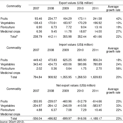
Yield increase in fruit crops (bananas and oranges) range around 53.0 percent to 58.0 percent; that of vegetables (onions and chilies) is around 64.0 percent to 65.0 percent4. Taking these results as they are is not quite enticing. Rather, it is more meaningful to look at the disparity between the yield under some scenarios and with no climate change/NoCC which would be assumed as due to the impact of climate change (bottom part of Table A1). This deserves further scrutiny. All other scenarios adopted in this paper forecast that the yields of bananas/oranges and chilies/onions would increase relative to those of NoCC scenario in 2050. The percentage changes in yield of the four climate change scenarios and of the NoCC scenario for 2050 are further summarized in Figures 1 for fruit crops and Figures 2 for vegetable crops.
Figure 1. Percentage Change in Fruit Crop Yield under Four Climate Change Scenarios, as Compared with No Climate Change (NoCC), 2050
Figure 2. Percentage Change in Vegetable Crop Yield under Four Climate Change Scenarios, as Compared with No Climate Change (NoCC), 2050
4
Impact on Production
National Aggregate Level
Fruits
Percentage changes in the production of bananas and oranges increased under all scenarios because bananas and oranges are combined as one commodity, tropical and sub-tropical fruits in the IFPRI’s IMPACT commodity list. The effect of the percentage changes on both crops is the same, because the percentage changes in yields are the same (Figures 1). Among the scenarios considered, 2050CSIRO_B1 gives the lowest percentage increase, and MIROC_B1 provides the highest. The percentage change increases range from 2.56 to 4.37 percent in 2050 (Figure 3). This conclusion does not appear to be in agreement with the results from the empirical study.
Figure 3. Percentage Change in Fruit Crop Production under Four Climate Change Scenarios, as Compared with No Climate Change, 2050
Vegetables
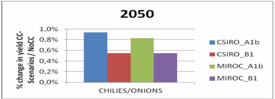
As in fruits, the projections for chilies and onions are the same—that is, percentage change in the production of onions and chilies increased under each scenario is equal. This is due to the fact that the magnitudes of yield change chilies and onions are the same, because they lump into one commodity, vegetables in the IFPRI’s IMPACT (Figures 2). Among the scenarios considered, CSIRO_B1 gives the lowest percentage increase, and MIROC_B1 provides the highest. The percentage change increases range from 0.57 to 1.29 percent in 2050 (Figure 4).
Regional Level
Fruits
The pattern of changes in the production of bananas and oranges across households is the same, because the yield changes are identical. For 2050, the model anticipates increases in the production of bananas and oranges by Java and Off-Java rural households, the percentage changes are estimated to be from 2.56 to 4.37 percent for both bananas/ oranges (Figure 5).
Figure 5. Percentage Change in Regional Household Production of Bananas and Oranges under Four Climate Change Scenarios, as Compared with No Climate Change, 2050
Vegetables
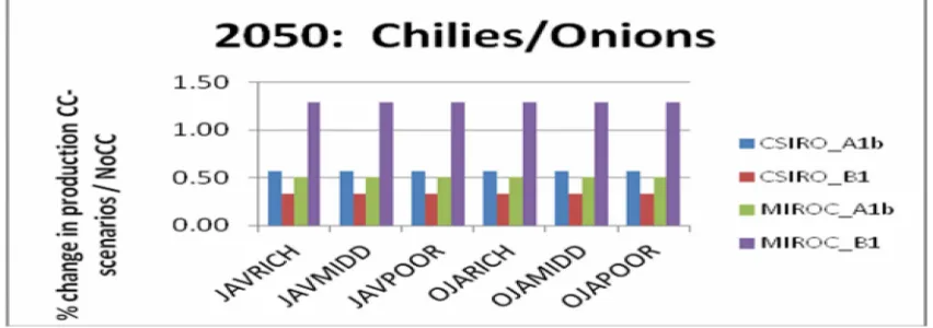
A similar pattern is observed in chili and onion production—that is, changes in the production of chilies and onions across households due to climate change by altering crop yields are the same, because the yield changes are also alike. For 2050, the model foresees increases in production for both chilies and onions by rural households in Java and Off-Java. The rates of these increases range from 0.33 to 1.29 percent (compared with NoCC) for both chillies/ onions (Figure 6).
Figure 6. Percentage Change in Regional Household Production of Chilies and Onions under Four Climate-Change Scenarios, as Compared with No Climate Change, 2050
change has been observed to cause material losses either at farm-level or regional level and is potential to drag the welfare of horticultural farmers down in the growing region (Padmasari 2010, Mayasari 2012). Average temperature increase in Batu town, an apple production center, was associated with falls in productivity and farm profits, in turns, apple farmers’ welfare (Mayasari 2012). In hot chili production center of Kediri district quantity and quality of produce was dropped due to excessive rainfall allegedly due to climate change during 2009 to 2011 (Maulidah et al. 20012).
Impact on Imports
Global climate change is a serious problem for human life around the world, because it affects all sectors of life. Growth in emissions is expected to have a severe and costly impact on Indonesia’s agriculture, infrastructure, biodiversity, and ecosystems, not to mention follow-on effects from the adverse impact of climate change on Indonesia’s neighbors in the Pacific and Asia. For example, in 2007, when Indonesia was experiencing too much rain, Indonesia had to import more than one million tons of milled rice. The relationship between the climate, crops, and the land is affected by radiation, rainfall, the availability of water, carbon dioxide, and air temperature (Oldeman et al. 1982). All of this, in turn, has an effect on nutrition.
In Indonesia, agriculture has received considerable attention because this sector is very sensitive to climate condition. Thus, agriculture has an important role to play in debates about adaptations needed to deal with climate change.
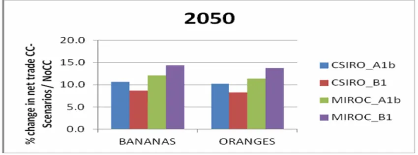
Fruits
In 2050, the percentage increases for bananas and oranges net trade are estimated to be much larger; bananas net trade range from 8.7 percent (Scenario CSIRO_B1) to 14.3 percent (Scenario MIROC_B1), and oranges net trade are 8.2 percent (Scenario CSIRO_B1) and 13.7 percent (Scenario MIROC_B1) (Figure 7).
Figure 7. Percentage Change in Fruit Crop Net Trade under Four Climate Change Scenarios, as Compared with No Climate Change, 2050 (Banana and Orange are Both Net Exports)
Vegetables
CSIRO_B1 and 4.1 percent for Scenario MIROC_B1 (Figure 8). As with oranges and bananas, these findings indicate that net trade of Onions and Chillies are not much affected by global climate change.
Figure 8. Percentage Change in Net Trade of Onions and Chilies under Four Climate Change Scenarios, as Compared with No Climate Change, 2050 (Chilies and Onions are Both Net Exports)
Impact on Consumption
Corresponding to changes in commodity production at the aggregate and household levels as a direct consequence of climate change, commodity available to the population will also adjust. This change, in turn, will instigate a change in per capita consumption.
Changes in Consumption Quantity at the National Aggregate Level
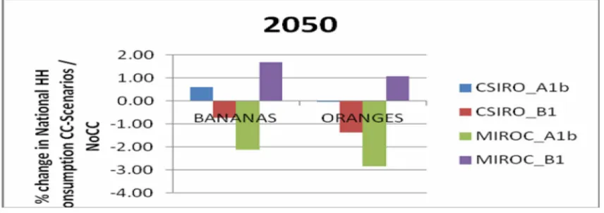
The results for changes in consumption quantity are mixed. Scenarios CSIRO_B1 and MIROC_A1b predict decreases in bananas and oranges consumption at rates between -0.73 and -2.85 percent, while Scenario MIROC_B1 foresees growth the consumption of them (Figure 9).
Figure 9. Percentage Change in National Household Consumption of Fruit Crops under Four Climate Change Scenarios, as Compared with No Climate Change, 2050
-3.78, whereas Scenario MIROC_B1 estimates an increase at 0.82 and 0.48, respectively (Figure 10).
Figure 10. Percentage Change in National Household Consumption of Vegetable Crops under Four Climate Change Scenarios, as Compared with No Climate Change, 2050
Changes in Consumption Quantity at the Regional Level
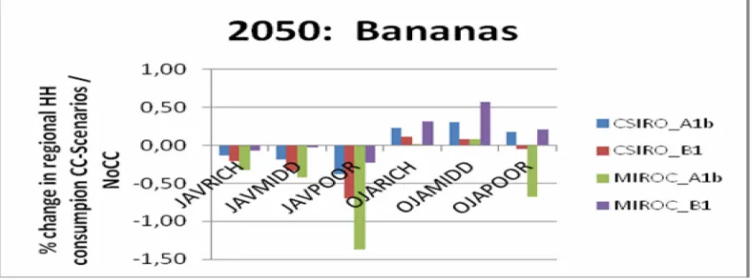
All model scenarios forecast that consumption of bananas in Java households will experience a decrease in 2050, from -0.02 to -1.37 percent. Java–poor households would suffer the most. On the other hand almost all types of Off-Java households will enjoy a positive rate of consumption changes, with the exception being the results of Scenario MIROC_A1b and Scenario CSIRO_B1 for Off-Java–poor households (Figure 11), which indicate a decrease in consumption ranging from -0.05 to -0.68 percent.
Figure 11. Percentage Change in Regional Household Consumption of Bananas under Four Climate Change Scenarios, as Compared with No Climate Change, 2050
Figure 12. Percentage Change in Regional Household Consumption of Oranges under Four Climate Change Scenarios, as Compared with No Climate Change, 2050
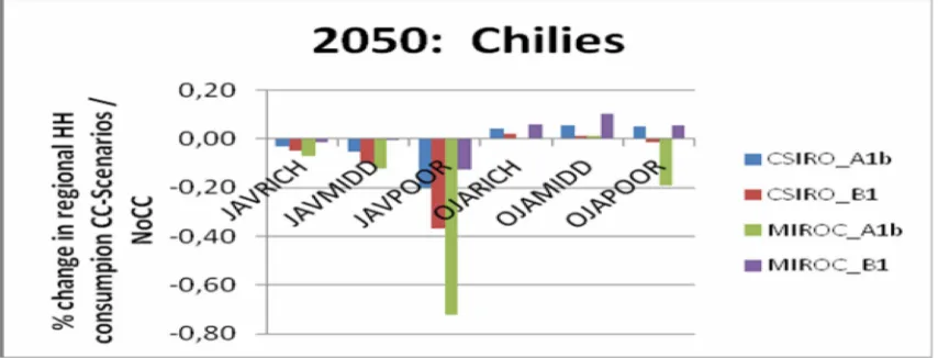
The rate of change of chilies consumption is also similar to that of bananas consumption. All scenarios show declining chilies consumption by Java households in 2050, ranging from -0.01 to -0.72 percent. Java–poor households would assume the greatest decreases, relative to other Java households. On the other hand, nearly all types of Off-Java households would benefit from positive rates of consumption changes ranging about 0.01 to 0.06 percents, with the exception being the results of Scenario CSIRO_B1 and MIROC_A1b (Figure 13) for Off-Java–poor households, which indicate a decrease in consumption ranging from -0.01 to -0.19 percent.
Figure 13. Percentage Change in Regional Household Consumption of Chilies under Four Climate Change Scenarios, as Compared with No Climate Change, 2050
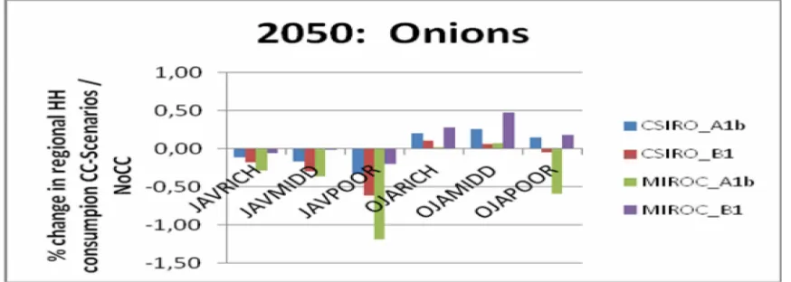
Figure 14. Percentage Change in Regional Household Consumption of Onions under Four Climate Change Scenarios, as Compared with No Climate Change, 2050
Ministry of Agriculture has also laid out some programs for adaptation to climate change (BAPPENAS 2009). These include the development of climate field school; integrated plant management field school; integrated pest control field school; development of soil cultivation technology and water-economical plant; building improved water storage; dissemination of compost-making devices; manure management to generate bio-energy; and adjustment in cropping pattern and diversifying production, application of high-yielding varieties that are adaptive and tolerant to drought, water submersion/flooding, salinity, resistant to pest and diseases, or short- or very-short matured (AARD 2011).
CONCLUSIONS AND POLICY RECOMMENDATIONS
All scenarios adopted by the IFPRI study predicts that the yields of fruit crop group (bananas and oranges) and vegetables (chilies and onions) would increase compared to the base scenarios. Notwithstanding, if comparison is made with no climate change /NoCC scenario, which is more meaningful, mixed conclusions are inevitable.
All other scenarios forecast that the yields of bananas/oranges and chilies/onions would increase relative to those of NoCC scenario. These yield increases or decreases will transform into enhancement or discouragement of total production of these respective commodities proportional to the combinations of parameters such as elasticities of yields with respect to their own prices, input prices, research and development, and changes in climate.
In regard to net trade indicator, this study foresees that bananas, oranges, chilies and onions imports would grow but the rate of growth in chilies and onions imports are not significant.
National consumption of bananas, oranges, chilies and onions are projected to fall under Scenarios CSIRO_B1 and MIROC_A1b but it increases under Scenario MIROC_B1. The model anticipates that there would be disparities of bananas, oranges, chilies and onions consumption among regions. Java households will experience decreases in consumption of these commodities in 2050, where Java–poor households would suffer the most. On the other hand almost all types of Off-Java households will enjoy a positive rate of consumption changes, with the exception being the results of Scenario MIROC_A1b and Scenario CSIRO_B1 for Off-Java–poor households, which indicate a decrease in consumption.
Climate change affects nearly all agricultural commodities, but food and horticultural crops and livestock are relatively more susceptible. However, the focus of adaptation in Indonesia today is more toward food crops and this is carried out by trailing the production of these crops with climate change. Adaptation technologies for fruits and orchard are limited only to mangoes, bananas, and papayas. For vegetables and estate crop, there is not much adaptation technologies available so far. This paper recommends that more researches on assembling cultivars that are adaptable or tolerable to drought as well as appropriate technologies to conserve water for horticultural crops and to use the limited amount of water efficiently are in high demand today. Best means to disseminate or communicate these cultivars and technologies to smallholder hgorticultural farmers ought to be explored.
REFERENCES
AARD (Agency for Agricultural Research and Development), Ministry of Agriculture/MoA, Indonesia. 2011. Pedoman Umum Adaptasi Perubahan Iklim Sektor Pertanian (General Guidelines for Adaptation to Climate Change in Agriculture). Jakarta.
www.litbang.deptan.go.id. (Accessed June 2011).
BAPPENAS (Badan Perencanaan Pembangunan Nasional). 2009. Indonesia Climate Change Sectoral Roadmap/ICCSR. Synthesis Report. 1st Edition. www.bappenas.go.id. (Accessed March 2011).
Boer, R. and A. Faqih. 2004. Current and Future Rainfall Variability in Indonesia. In An Integrated Assessment of Climate Change Impacts, Adaptation and Vulnerability in Watershed Areas and Communities in Southeast Asia, Repor t from AIACC Project No. AS21 (Annex C, 95-126). International START Secretariat, Washington, District of Columbia. http://sedac.ciesin.org/aiac c/progress/FinalRept_AIACC_AS21.pdf . (Accessed Desember 2010).
Case, M., F. Ardiansyah, and E. Spector. On-line 2012. Climate Change in Indonesia: Implications for Humans and Nature. http://assets.wwf.org.uk/downloads/indonesian_climate_ch.pdf. (Accessed Desember 2011).
The Copenhagen Diagnosis. On-line 2012. The Copenhagen Diagnosis: Climate Science Report , p. 36.http://www.copenhagendiagnosis.org/. (Accessed January 2012).
CRU (Climatic Research Unit), UEA (University of East Anglia). On-line 2012. Temperature.
http://www.cru.uea.ac.uk/cru/data/temperature/. (Accessed January 2012).
GISS (Goddard Institute for Space Studies), NASA (National Aeronautics and Space Administration). On-line 2012. GISS Surface Temperature Analysis (GISTEMP).
http://data.giss.nasa.gov/gistemp/. (Accessed January 2012).
Maulidah, S. , H. Santoso, H. Subagyo, Q. Rifqiyyah. 2012. Dampak Perubahan Iklim terhadap Produksi dan Pendapatan Usaha Tani Cabai Rawit. SEPA : Vol. 8 No. 2 Pebruari 2012 : 51 – 182. http://agribisnis.fp.uns.ac.id/wp-content/uploads/2012/10/Jurnal-SEPA-137- DAMPAK-PERUBAHAN-IKLIM-TERHADAP-PRODUKSI-DAN-PENDAPATAN-USAHA-TANI-CABAI-RAWIT.pdf. (Accessed January 2012).
Mayasari, S. P. 2012. Identifikasi Opsi Adaptasi Perubahan Iklim bagi Petani Apel di Kota Batu, Jawa Timur (Studi Kasus: Desa Bumiaji, Kecamatan Bumiaji). Abstraksi.
http://sappk.lib.itb.ac.id/index.php?menu=library&action=detail&libraryID=18291. (Accessed January 2012).
NASA. 2012. Global Climate Change: Vital Signs of the Planet. National Aeronautics and Space Administration/NASA.http://climate.nasa.gov/evidence. (Accessed January 2012).
NCDC (National Climatic Data Center), NOAA (National Oceanic and Atmospheric Administration). On-line 2012. Global Surface Temperature Anomalies. http://www.ncdc.noaa.gov/cmb-faq/anomalies.php#mean. (Accessed January 2012).
Nelson, G. C., M. W. Rosegrant, J. Koo, R. Robertson, T. Sulser, T. Zhu, C. Ringler, S. Msangi, A. Palazzo, M. Batka, M. Magalhaes, R. Valmonte-Santos, M. Ewing, and D. Lee. 2009. Impact on Agriculture and Costs of Adaptation. Food Policy Report. Washington DC: International Food Policy Research Institute.www.ifpri.org. (Accessed March 2010). NSIDC (National Snow and Ice Data Center). On-line 2012. Glaciers.
http://nsidc.org/cryosphere/sotc/glacier_balance.html. (Accessed January 2012).
Oldeman. L. R and M. Prere 1982. A Study of the Agroclimatology of the Humid Tropics of the Southeast Asia. FAO of United Nation Rome.
Padmasari, C. 2010. Respon Petani Hortikultura terhadap Dampak Perubahan Iklim: Studi Kasus: Desa Margamukti, Pengalengan. Abstraksi. http://sappk.lib.itb.ac.id/index.php?menu= library&action=detail&libraryID=16177. (Accessed January 2012).
PMEL (Pacific Marine Environmental Laboratory), NOAA. On-line 2012. Carbon Dioxide Program.
http://www.pmel.noaa.gov/co2/story/What+is+Ocean+Acidification%3F. (Accessed
January 2012).
PMEL (Pacific Marine Environmental Laboratory), NOAA. On-line 2012. Ocean Acidification: The Other Carbon Dioxide Problem. .http://www.pmel.noaa.gov/co2/story/Ocean+Acidification.
(Accessed January 2012).
PEACE (PT. Pelangi Energi Abadi Citra Enviro). 2007. Executive Summary: Indonesia and Climate Change. Working Paper on Current Status and Policies. PT. Pelangi Energi Abadi Citra Enviro.www.peace.co.id. (Accessed December 2010).
Sayaka, B., Sumaryanto, A. Croppenstedt, and S. DiGiuseppe. 2007a. An Assessment of the Impact of Rice Tariff Policy in Indonesia: A Multi-Market Model Approach. Agricultural Development Economics Division (ESA) Working Paper 07-18. Food and Agriculture Organization, Agricultural Development Economics Division, Rome. www.fao.org/es/esa. (Accessed April 2010).
Sayaka, B. Sumaryanto, M. Siregar, A. Croppenstedt, and S. DiGiuseppe. 2007b. An Assessment of the Impact of Higher Yields for Maize, Soybean and Cassava in Indonesia: A Multi-Market Model Approach. Agricultural Development Economics Division (ESA) Working Paper 07-25. Food and Agriculture Organization, Agricultural Development Economics Division, Rome.www.fao.org/es/esa. (Accessed November 2009).
Stifel, D., and J.-C. Randrianarisoa. 2004. “Rice Prices, Agricultural Input Subsidies, Transactions Costs, and Seasonality: A Multi-Market Model Poverty and Social Impact Analysis (PSIA) for Madagascar.” stifel_david_juillet_8. (Accessed February 2011).
Tsonis, A.A., Elsner, J.B., Hunt, A.G., and Jagger, T. H. 2005. Unfolding the Relation between Global Temperature and ENSO. Geophysical Research Letters 32, L09701, doi:10.1029/ 2005GL022875. (Accessed Desember 2011).
Table 1. Changes in Crop Yields under Various Scenarios (Percent Increase)
Compared to Base Year in 2050 Selected Crops
CSIRO_A1b CSIRO_B1 MIROC_A1b MIROC_B1 NoCC
BANANAS 57.5% 56.5% 58.0% 59.3% 52.6%
ORANGES 57.5% 56.5% 58.0% 59.3% 52.6%
ONIONS 65.3% 64.9% 65.2% 66.5% 64.3%
CHILIES 65.3% 64.9% 65.2% 66.5% 64.3%
Compared to No Climate/NoCC scenario in 2050 Selected Crops
CSIRO_A1b CSIRO_B1 MIROC_A1b MIROC_B1
BANANAS 4,92% 3,90% 5,35% 3,90%
ORANGES 4,92% 3,90% 5,35% 3,90%
ONIONS 0,94% 0,55% 0,83% 0,55%
CHILIES 0,94% 0,55% 0,83% 0,55%