Tools for Signal
Compression
First published 2011 in Great Britain and the United States by ISTE Ltd and John Wiley & Sons, Inc. Adapted and updated from Outils pour la compression des signaux: applications aux signaux audioechnologies du stockage d’énergie published 2009 in France by Hermes Science/Lavoisier © Institut Télécom et LAVOISIER 2009
Apart from any fair dealing for the purposes of research or private study, or criticism or review, as permitted under the Copyright, Designs and Patents Act 1988, this publication may only be reproduced, stored or transmitted, in any form or by any means, with the prior permission in writing of the publishers, or in the case of reprographic reproduction in accordance with the terms and licenses issued by the CLA. Enquiries concerning reproduction outside these terms should be sent to the publishers at the undermentioned address:
ISTE Ltd John Wiley & Sons, Inc. 27-37 St George’s Road 111 River Street
London SW19 4EU Hoboken, NJ 07030
UK USA
www.iste.co.uk www.wiley.com
© ISTE Ltd 2011
The rights of Nicolas Moreau to be identified as the author of this work have been asserted by him in accordance with the Copyright, Designs and Patents Act 1988.
____________________________________________________________________________________ Library of Congress Cataloging-in-Publication Data
Moreau, Nicolas, 1945-
[Outils pour la compression des signaux. English] Tools for signal compression / Nicolas Moreau. p. cm.
"Adapted and updated from Outils pour la compression des signaux : applications aux signaux audioechnologies du stockage d'energie."
Includes bibliographical references and index. ISBN 978-1-84821-255-8
1. Sound--Recording and reproducing--Digital techniques. 2. Data compression (Telecommunication) 3. Speech processing systems. I. Title.
TK7881.4.M6413 2011 621.389'3--dc22
2011003206 British Library Cataloguing-in-Publication Data
A CIP record for this book is available from the British Library ISBN 978-1-84821-255-8
Introduction . . . xi
PART1. TOOLS FORSIGNALCOMPRESSION . . . 1
Chapter 1. Scalar Quantization . . . 3
1.1. Introduction . . . 3
1.2. Optimum scalar quantization . . . 4
1.2.1. Necessary conditions for optimization . . . 5
1.2.2. Quantization error power . . . 7
1.2.3. Further information . . . 10
1.2.3.1. Lloyd–Max algorithm . . . 10
1.2.3.2. Non-linear transformation . . . 10
1.2.3.3. Scale factor . . . 10
1.3. Predictive scalar quantization . . . 10
1.3.1. Principle . . . 10
1.3.2. Reminders on the theory of linear prediction . . . 12
1.3.2.1. Introduction: least squares minimization . . . 12
1.3.2.2. Theoretical approach . . . 13
1.3.2.3. Comparing the two approaches . . . 14
1.3.2.4. Whitening filter . . . 15
1.3.2.5. Levinson algorithm . . . 16
1.3.3. Prediction gain . . . 17
1.3.3.1. Definition . . . 17
1.3.4. Asymptotic value of the prediction gain . . . 17
1.3.5. Closed-loop predictive scalar quantization . . . 20
Chapter 2. Vector Quantization . . . 23
2.1. Introduction . . . 23
2.3. Optimum codebook generation . . . 26
2.4. Optimum quantizer performance . . . 28
2.5. Using the quantizer . . . 30
2.5.1. Tree-structured vector quantization . . . 31
2.5.2. Cartesian product vector quantization . . . 31
2.5.3. Gain-shape vector quantization . . . 31
2.5.4. Multistage vector quantization . . . 31
2.5.5. Vector quantization by transform . . . 31
2.5.6. Algebraic vector quantization . . . 32
2.6. Gain-shape vector quantization . . . 32
2.6.1. Nearest neighbor rule . . . 33
2.6.2. Lloyd–Max algorithm . . . 34
Chapter 3. Sub-band Transform Coding . . . 37
3.1. Introduction . . . 37
3.2. Equivalence of filter banks and transforms . . . 38
3.3. Bit allocation . . . 40
3.3.1. Defining the problem . . . 40
3.3.2. Optimum bit allocation . . . 41
3.3.3. Practical algorithm . . . 43
3.3.4. Further information . . . 43
3.4. Optimum transform . . . 46
3.5. Performance . . . 48
3.5.1. Transform gain . . . 48
3.5.2. Simulation results . . . 51
Chapter 4. Entropy Coding . . . 53
4.1. Introduction . . . 53
4.2. Noiseless coding of discrete, memoryless sources . . . 54
4.2.1. Entropy of a source . . . 54
4.2.2. Coding a source . . . 56
4.2.2.1. Definitions . . . 56
4.2.2.2. Uniquely decodable instantaneous code . . . 57
4.2.2.3. Kraft inequality . . . 58
4.2.2.4. Optimal code . . . 58
4.2.3. Theorem of noiseless coding of a memoryless discrete source . . . 60
4.2.3.1. Proposition 1 . . . 60
4.2.3.2. Proposition 2 . . . 61
4.2.3.3. Proposition 3 . . . 61
4.2.3.4. Theorem . . . 62
4.2.4. Constructing a code . . . 62
4.2.4.2. Huffman algorithm . . . 63
4.2.4.3. Example 1 . . . 63
4.2.5. Generalization . . . 64
4.2.5.1. Theorem . . . 64
4.2.5.2. Example 2 . . . 65
4.2.6. Arithmetic coding . . . 65
4.3. Noiseless coding of a discrete source with memory . . . 66
4.3.1. New definitions . . . 67
4.3.2. Theorem of noiseless coding of a discrete source with memory . . . 68
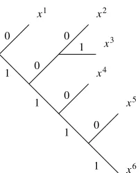
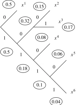
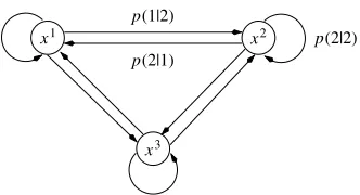
4.3.3. Example of a Markov source . . . 69
4.3.3.1. General details . . . 69
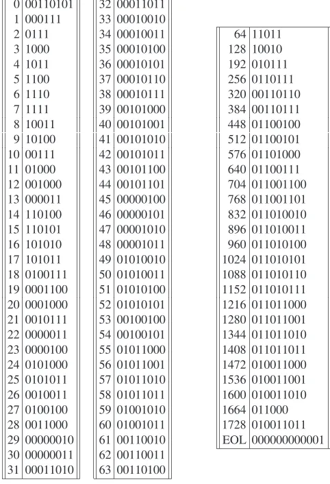
4.3.3.2. Example of transmitting documents by fax . . . 70
4.4. Scalar quantizer with entropy constraint . . . 73
4.4.1. Introduction . . . 73
4.4.2. Lloyd–Max quantizer . . . 74
4.4.3. Quantizer with entropy constraint . . . 75
4.4.3.1. Expression for the entropy . . . 76
4.4.3.2. Jensen inequality . . . 77
4.4.3.3. Optimum quantizer . . . 78
4.4.3.4. Gaussian source . . . 78
4.5. Capacity of a discrete memoryless channel . . . 79
4.5.1. Introduction . . . 79
4.5.2. Mutual information . . . 80
4.5.3. Noisy-channel coding theorem . . . 82
4.5.4. Example: symmetrical binary channel . . . 82
4.6. Coding a discrete source with a fidelity criterion . . . 83
4.6.1. Problem . . . 83
4.6.2. Rate–distortion function . . . 84
4.6.3. Theorems . . . 85
4.6.3.1. Source coding theorem . . . 85
4.6.3.2. Combined source-channel coding . . . 85
4.6.4. Special case: quadratic distortion measure . . . 85
4.6.4.1. Shannon’s lower bound for a memoryless source . . . 85
4.6.4.2. Source with memory . . . 86
4.6.5. Generalization . . . 87
PART2. AUDIOSIGNALAPPLICATIONS . . . 89
Chapter 5. Introduction to Audio Signals . . . 91
5.1. Speech signal characteristics . . . 91
5.2. Characteristics of music signals . . . 92
5.3.1. Telephone-band speech signals . . . 93
5.3.1.1. Public telephone network . . . 93
5.3.1.2. Mobile communication . . . 94
5.3.1.3. Other applications . . . 95
5.3.2. Wideband speech signals . . . 95
5.3.3. High-fidelity audio signals . . . 95
5.3.3.1. MPEG-1 . . . 96
5.3.3.2. MPEG-2 . . . 96
5.3.3.3. MPEG-4 . . . 96
5.3.3.4. MPEG-7 and MPEG-21 . . . 99
5.3.4. Evaluating the quality . . . 99
Chapter 6. Speech Coding . . . 101
6.1. PCM and ADPCM coders . . . 101
6.2. The 2.4 bit/s LPC-10 coder . . . 102
6.2.1. Determining the filter coefficients . . . 102
6.2.2. Unvoiced sounds . . . 103
6.2.3. Voiced sounds . . . 104
6.2.4. Determining voiced and unvoiced sounds . . . 106
6.2.5. Bit rate constraint . . . 107
6.3. The CELP coder . . . 107
6.3.1. Introduction . . . 107
6.3.2. Determining the synthesis filter coefficients . . . 109
6.3.3. Modeling the excitation . . . 111
6.3.3.1. Introducing a perceptual factor . . . 111
6.3.3.2. Selecting the excitation model . . . 113
6.3.3.3. Filtered codebook . . . 113
6.3.3.4. Least squares minimization . . . 115
6.3.3.5. Standard iterative algorithm . . . 116
6.3.3.6. Choosing the excitation codebook . . . 117
6.3.3.7. Introducing an adaptive codebook . . . 118
6.3.4. Conclusion . . . 121
Chapter 7. Audio Coding . . . 123
7.1. Principles of “perceptual coders” . . . 123
7.2. MPEG-1 layer 1 coder . . . 126
7.2.1. Time/frequency transform . . . 127
7.2.2. Psychoacoustic modeling and bit allocation . . . 128
7.2.3. Quantization . . . 128
7.3. MPEG-2 AAC coder . . . 130
7.4. Dolby AC-3 coder . . . 134
7.5. Psychoacoustic model: calculating a masking threshold . . . 135
7.5.2. The ear . . . 135
7.5.3. Critical bands . . . 136
7.5.4. Masking curves . . . 137
7.5.5. Masking threshold . . . 139
Chapter 8. Audio Coding: Additional Information . . . 141
8.1. Low bit rate/acceptable quality coders . . . 141
8.1.1. Tool one: SBR . . . 142
8.1.2. Tool two: PS . . . 143
8.1.2.1. Historical overview . . . 143
8.1.2.2. Principle of PS audio coding . . . 143
8.1.2.3. Results . . . 144
8.1.3. Sound space perception . . . 145
8.2. High bit rate lossless or almost lossless coders . . . 146
8.2.1. Introduction . . . 146
8.2.2. ISO/IEC MPEG-4 standardization . . . 147
8.2.2.1. Principle . . . 147
8.2.2.2. Some details . . . 147
Chapter 9. Stereo Coding: A Synthetic Presentation . . . 149
9.1. Basic hypothesis and notation . . . 149
9.2. Determining the inter-channel indices . . . 151
9.2.1. Estimating the power and the intercovariance . . . 151
9.2.2. Calculating the inter-channel indices . . . 152
9.2.3. Conclusion . . . 154
9.3. Downmixing procedure . . . 154
9.3.1. Development in the time domain . . . 155
9.3.2. In the frequency domain . . . 157
9.4. At the receiver . . . 158
9.4.1. Stereo signal reconstruction . . . 158
9.4.2. Power adjustment . . . 159
9.4.3. Phase alignment . . . 160
9.4.4. Information transmitted via the channel . . . 161
9.5. Draft International Standard . . . 161
PART3. MATLAB PROGRAMS . . . . 163
Chapter 10. A Speech Coder . . . 165
10.1. Introduction . . . 165
10.2. Script for the calling function . . . 165
Chapter 11. A Music Coder . . . 173
11.1. Introduction . . . 173
11.2. Script for the calling function . . . 173
11.3. Script for called functions . . . 176
Bibliography . . . 195
In everyday life, we often come in contact with compressed signals: when using mobile telephones, mp3 players, digital cameras, or DVD players. The signals in each of these applications, telephone-band speech, high fidelity audio signal, and still or video images are not only sampled and quantized to put them into a form suitable for saving in mass storage devices or to send them across networks, but also compressed. The first operation is very basic and is presented in all courses and introductory books on signal processing. The second operation is more specific and is the subject of this book: here, the standard tools for signal compression are presented, followed by examples of how these tools are applied in compressing speech and musical audio signals. In the first part of this book, we focus on a problem which is theoretical in nature: minimizing the mean squared error. The second part is more concrete and qualifies the previous steps in seeking to minimize the bit rate while respecting the psychoacoustic constraints. We will see that signal compression consists of seeking not only to eliminate all redundant parts of the original signal but also to attempt the elimination of inaudible parts of the signal.
The compression techniques presented in this book are not new. They are explained in theoretical framework, information theory, and source coding, aiming to formalize the first (and the last) element in a digital communication channel: the encoding of an analog signal (with continuous times and continuous values) to a digital signal (at discrete times and discrete values). The techniques come from the work by C. Shannon, published at the beginning of the 1950s. However, except for the development of speech encodings in the 1970s to promote an entirely digitally switched telephone network, these techniques really came into use toward the end of the 1980s under the influence of working groups, for example, “Group Special Mobile (GSM)”, “Joint Photographic Experts Group (JPEG)”, and “Moving Picture Experts Group (MPEG)”.
a music signal. We know that a music signal can be reconstructed with quasi-perfect quality (CD quality) if it was sampled at a frequency of 44.1 kHz and quantized at a resolution of 16 bits. When transferred across a network, the required bit rate for a mono channel is 705 kb/s. The most successful audio encoding, MPEG-4 AAC, ensures “transparency” at a bit rate of the order of 64 kb/s, giving a compression rate greater than 10, and the completely new encoding MPEG-4 HE-AACv2, standardized in 2004, provides a very acceptable quality (for video on mobile phones) at 24 kb/s for 2 stereo channels. The compression rate is better than 50!
In the Part 1 of this book, the standard tools (scalar quantization, predictive quantization, vector quantization, transform and sub-band coding, and entropy coding) are presented. To compare the performance of these tools, we use an academic example of the quantization of the realization x(n) of a one-dimensional random process X(n). Although this is a theoretical approach, it not only allows objective assessment of performance but also shows the coherence between all the available tools. In the Part 2, we concentrate on the compression of audio signals (telephone-band speech, wide(telephone-band speech, and high fidelity audio signals).
Throughout this book, we discuss the basic ideas of signal processing using the following language and notation. We consider a one-dimensional, stationary, zero-mean, random process X(n), with power σ2
X and power spectral density SX(f). We also assume that it is Gaussian, primarily because the Gaussian distribution is preserved in all linear transformations, especially in a filter which greatly simplifies the notation, and also because a Gaussian signal is the most difficult signal to encode because it carries the greatest quantization error for any bit rate. A column vector ofN dimensions is denoted byX(m)and constructed withX(mN)· · ·X(mN+N−1). These N random variables are completely defined statistically by their probability density function: whereRXis the autocovariance matrix:
RX=E{X(m)Xt(m)}= Toeplitz matrix with N ×N dimensions. Moreover, we assume an auto-regressive process X(n)of order P, obtained through filtering with white noiseW(n) with variance σ2
W via a filter of order P with a transfer function 1/A(z) for A(z) in the form:
The purpose of considering the quantization of an auto-regressive waveform as our example is that it allows the simple explanation of all the statistical characteristics of the source waveform as a function of the parameters of the filter such as, for example, the power spectral density:
SX(f) = σ 2 W |A(f)|2
Scalar Quantization
1.1. Introduction
Let us consider a discrete-time signalx(n)with values in the range[−A,+A]. Defining a scalar quantization with a resolution ofb bits per sample requires three operations:
– partitioning the range [−A,+A] into L = 2b non-overlapping intervals
{Θ1· · ·ΘL}of length{∆1· · ·∆L},
– numbering the partitioned intervals{i1· · ·iL},
– selecting the reproduction value for each interval, the set of these reproduction values forms a dictionary (codebook)1C={xˆ1· · ·xˆL}.
Encoding (in the transmitter) consists of deciding which intervalx(n) belongs to and then associating it with the corresponding number i(n) ∈ {1· · ·L = 2b}. It is the number of the chosen interval, the symbol, which is transmitted or stored. The decoding procedure (at the receiver) involves associating the corresponding reproduction value x(n) = ˆˆ xi(n) from the set of reproduction values {xˆ1· · ·xˆL} with the numberi(n). More formally, we observe that quantization is a non-bijective mapping to[−A,+A]in a finite setCwith an assignment rule:
ˆ
x(n) = ˆxi(n)∈ {xˆ1· · ·xˆL} iff x(n)∈Θi
The process is irreversible and involves loss of information, a quantization error which is defined as q(n) = x(n)−x(n)ˆ . The definition of a distortion measure
d[x(n),x(n)]ˆ is required. We use the simplest distortion measure, quadratic error: d[x(n),x(n)] =ˆ |x(n)−x(n)ˆ |2
This measures the error in each sample. For a more global distortion measure, we use the mean squared error (MSE):
D=E{|X(n)−x(n)ˆ |2}
This error is simply denoted as the quantization error power. We use the notation σ2
Qfor the MSE.
Figure 1.1(a) shows, on the left, the signal before quantization and the partition of the range[−A,+A]whereb= 3, and Figure 1.1(b) shows the reproduction values, the reconstructed signal and the quantization error. The bitstream between the transmitter and the receiver is not shown.
5 10 15 20 25 30 35 40 45 50 –8
–6 –4 –2 0 2 4 6 8
5 10 15 20 25 30 35 40 45 50 –8
–6 –4 –2 0 2 4 6 8
(a) (b)
Figure 1.1.(a) The signal before quantization and the partition of the range
[−A,+A]and (b) the set of reproduction values, reconstructed signal, and quantization error
The problem now consists of defining the optimal quantization, that is, in defining the intervals{Θ1· · ·ΘL}and the set of reproduction values{xˆ1· · ·xˆL}to minimizeσ2
Q.
1.2. Optimum scalar quantization
processX(n)takes at timen. No other direct use of the correlation that exists between the values of the process at different times is possible. It is enough to know the marginal probability density function ofX(n), which is written aspX(.).
1.2.1. Necessary conditions for optimization
To characterize the optimum scalar quantization, the range partition and reproduction values must be found which minimize:
σQ2 =E{[X(n)−x(n)]ˆ 2}= L
i=1 u∈Θi
(u−xˆi)2pX(u)du [1.1]
This joint minimization is not simple to solve. However, the two necessary conditions for optimization are straightforward to find. If the reproduction values {ˆx1· · ·xˆL} are known, the best partition {Θ1· · ·ΘL} can be calculated. Once the partition is found, the best reproduction values can be deduced. The encoding part of quantization must be optimal if the decoding part is given, and vice versa. These two necessary conditions for optimization are simple to find when the squared error is chosen as the measure of distortion.
– Condition 1: Given a codebook{ˆx1· · ·xˆL}, the best partition will satisfy: Θi={x: (x−xˆi)2≤(x−xˆj)2 ∀j ∈ {1· · ·L} }
This is the nearest neighbor rule.
If we definetisuch that it defines the boundary between the intervalsΘiandΘi+1, minimizing the MSEσ2
Qrelative totiis found by noting:
∂ ∂ti
ti
ti−1
(u−xˆi)2pX(u)du+ ti+1
ti
(u−xˆi+1)2pX(u)du
= 0
(ti−xˆi)2p
X(ti)−(ti−xˆi+1)2pX(ti) = 0 such that:
ti= xˆi+ ˆxi+1 2
– Condition 2: Given a partition {Θ1· · ·ΘL}, the optimum reproduction values are found from the centroid (or center of gravity) of the section of the probability density function in the region ofΘi:
ˆ xi=
u∈ΘiupX(u)du
u∈ΘipX(u)du
First, note that minimizingσ2
Qrelative toxˆiinvolves only an element from the sum given in [1.1]. From the following:
∂ ∂ˆxi
u∈Θi
(u−xˆi)2p
X(u)du= 0
−2 u∈Θi
upX(u)du+ 2ˆxi u∈Θi
pX(u)du= 0 we find the first identity of equation [1.2].
Since:
u∈Θi
upX(u)du= u∈Θi
pX(u)du ∞
−∞
upX|Θi(u)du
wherepX|Θiis the conditional probability density function ofX, whereX ∈Θi, we find:
ˆ xi=
∞
−∞
upX|Θi(u)du
ˆ
xi=E{X|X ∈Θi}
The required value is the mean value ofX in the interval under consideration.2
It can be demonstrated that these two optimization conditions are not sufficient to guarantee optimized quantization except in the case of a Gaussian distribution.
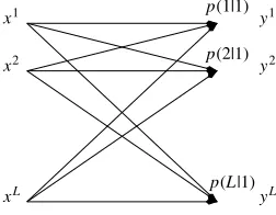
Note that detailed knowledge of the partition is not necessary. The partition is determined entirely by knowing the distortion measure, applying the nearest neighbor rule, and from the set of reproduction values. Figure 1.2 shows a diagram of the encoder and decoder.
x1 ... xL x1 ... xL
i(n)
x(n) Look up x(n)
in a table Nearest
neighbor rule
Figure 1.2.Encoder and decoder
1.2.2. Quantization error power
When the numberLof levels of quantization is high, the optimum partition and the quantization error power can be obtained as a function of the probability density functionpX(x), unlike in the previous case. This hypothesis, referred to as the
high-resolutionhypothesis, declares that the probability density function can be assumed to be constant in the interval[ti−1, ti]and that the reproduction value is located at the middle of the interval. We can therefore write:
pX(x)≈pX(ˆxi) for x∈[ti−1, ti]
ˆ
xi≈ ti−1+ti 2
We define the length of the interval as:
∆(i) =ti−ti−1 for an interval[ti−1, ti]and:
Pprob(i) =Pprob{X ∈[ti−1, ti]}=pX(ˆxi)∆(i)
is the probability thatX(n)belongs to the interval[ti−1, ti]. The quantization error power is written as:
σQ2 =
This is also written as:
σQ2 =
The quantization error power depends only on the length of the intervals∆(i). We are looking for{∆(1)· · ·∆(L)}such thatσ2
Qis minimized. Let:
As:
since this integral is now independent of∆(i), we minimize the sum of the cubes of Lpositive numbers with a constant sum. This is satisfied with numbers that are all equal. Hence, we have:
α(1) =· · ·=α(L) which implies:
α3(1) =· · ·=α3(L)
pX(ˆx1)∆3(1) =· · ·=pX(ˆxL)∆3(L)
The relation means that an interval is even smaller, that the probability thatX(n) belongs to this interval is high, and that all the intervals contribute equally to the quantization error power. The expression for the quantization error power is:
σQ2 =
SinceL= 2b, we obtain what is known as the Bennett formula:
σQ2 =
This demonstration is not mathematically rigorous. It will be discussed at the end of Chapter 4 where we compare this mode of quantization with what is known as quantization with entropy constraint.
Note that the explanation via Bennett’s formula is not necessary. We can obtain this result directly!
For a Gaussian zero-mean signal, with powerσ2
X, for which: From this, we deduce that:
σ2
This equation is referred to throughout this book. From this, we can write the equivalent expression:
From this we deduce the 6 dB per bit rule. We can show that for all other distributions (Laplacian, etc.), the minimum quantization error power is always between these two values. The case of the uniformly distributed signal is more favorable, whereas the Gaussian case is less favorable. Shannon’s work and the rate/distortion theory affirm this observation.
1.2.3. Further information
1.2.3.1. Lloyd–Max algorithm
In practice,pX(x)is unknown. To construct a quantizer, we use empirical data, assign the same weight to each value and apply the Lloyd–Max algorithm in the so-called Linde-Buzo-Gray (LBG) form. This algorithm, which is generalized for vector quantization, is presented in the following chapter.
1.2.3.2. Non-linear transformation
A non-uniform scalar quantizer can be seen as a uniform scalar quantizer that has been preceded by a nonlinear transformation and followed with the inverse transformation.3 The transformation is defined by its characteristic f(x). From this perspective, the problem consists of choosing the non-linear transformation which minimizes the quantization error power. This forms the subject of important developments in two works by: Jayant and Noll [JAY 84] and Gersho and Gray [GER 92]. This development no longer seems to be of great importance because vector quantization became the basic tool of choice.
1.2.3.3. Scale factor
During a quantization operation on real signals (speech, music, and pictures), it is important to estimate the parameterAwhich varies with time; real signals do not satisfy the stationarity hypothesis! We examine this problem in the following chapter by introducing a special quantization called gain shapewhich is particularly well adapted to signals with significant instantaneous changes in power, for example, audio signals.
1.3. Predictive scalar quantization
1.3.1. Principle
In the preceding exposition, we saw that during quantization, no other use is made with the statistical links between successive values of the signal. We will see that predictive scalar quantization aims to decorrelate the signal before quantizing it and that the use of correlation improves the general behavior of the system, that is, it reduces the quantization error power.
An outline of the principle of predictive scalar quantization is shown in Figure 1.3. We subtract a new signal v(n)from the signalx(n). Next, we perform the encoding/decoding procedure on the signaly(n) =x(n)−v(n). At the decoder, we addv(n)back to the reconstructed signal valuesˆy(n).
Q Q–1
y(n) x(n) +
+
–
+ +
+
x(n) y(n)
v(n)
A′(z)
Figure 1.3.Outline of the principle of predictive scalar quantization
We can immediately see that, in a real-world application of coding, this scheme is not very realistic since the signalv(n)must also be transmitted to the decoder, but let us wait until the end of the chapter before demonstrating how we go from aopen-loop
scheme to a more realistic, but more complicated to analyze,closed-loopscheme.
If we subtract a value from the signal before encoding it and add it back after decoding, the quantization errorq(n) =y(n)−y(n)ˆ and reconstruction errorq(n) =¯ x(n)−x(n)ˆ must always be equal because:
q(n) =y(n)−y(n) =ˆ x(n)−v(n)−[ˆx(n)−v(n)] = ¯q(n)
Hence their respective powers are identical. Since the main interest of the user of the complete system is to have the smallest possible reconstruction error power, the problem becomes simply the reduction of the quantization error power. If we assume an optimized scalar quantization ofy(n), we know that the quantization error power can be expressed as:
σQ2 =c σY2 2−2b
From this, we conclude that seeking to minimize the reconstruction error powerσ2 ¯ Q leads us back to minimizeσ2
Y fromy(n).
We have a great range of choices forv(n). If we takev(n)in the form:
v(n) =−
P
i=1
aix(n−i)
while introducingPparameters, we speak oflinear prediction of orderP. The signal y(n)is the prediction error which is expressed as:
y(n) =x(n)−v(n) =x(n) + P
i=1
The relationship between x(n) and y(n) is that of a transfer function filtering operation4:
B(z) = 1 +a1z−1+· · ·+aPz−P Minimizingσ2
Y concerns the coefficients of this predictive filter.
This problem has been the subject of numerous studies since 1960s. All modern books that present basic techniques for signal processing include a chapter on this problem, for example [KAY 88]. In this book, we set out a few reminders.
1.3.2. Reminders on the theory of linear prediction
1.3.2.1. Introduction: least squares minimization
Since this theory, which can be used in numerous signal processing applications, was developed quite rightly with the goal of determining a method of speech coding with reduced rates and, in coding speech, the method uses a block of N samples,5 the problem can be posed in the following way: knowingx = [x(0)· · ·x(N−1)]t determinea = [a1· · ·aP]twhile minimizing the empirical power of the prediction error:
4. Despite using the same notation to avoid overwhelming the reader, we must not confuse the coefficientsaiand the orderPof the generating filter ofx(n)with the coefficients and the order
of the predictor polynomial. Throughout this chapter, we are only concerned with the predictor filter.
we can write:
The vectoraoptis that which satisfies:
∂ The minimum can be written as:
ˆ
Let us assume that the signal x(n) can be interpreted (modeled) as the realization of a stationary random process with an autocovariance functionrX(k) = E{X(n)X(n−k)}. We need to find the vectorawhich minimizes the prediction
Y relative toainvolves thenormal equations:
Raopt=−r
and as the autocovariance matrixRis definite-positive (except for the limiting case whereX(n)is an harmonic random process), it is invertible. We therefore have:
We also have:
(σY2)min=σX2 + 2(aopt)tr−(aopt)tr=σ2X+ (aopt)tr [1.7] Note that these two equations together [1.6] and [1.7] allow the unique matrix representation:
1.3.2.3. Comparing the two approaches
The two solutions are comparable, which is unsurprising because1/NΓtxis an estimate of the vector rand1/NΓtΓis an estimate ofR. More precisely, the two approaches are asymptotically equivalent since, when the signalX(n)is an ergodic random process, that is, if:
lim
The difference (essential but subtle) is that since the exact covariance matrix is definite-positive (except in the limiting case where the process is harmonic), it is always invertible while the matrixΓtΓ(expressed here withP = 1for simplicity):
x2(1) +· · ·x2(N−2) x(0)x(1) +· · ·+x(N −3)x(N−2) x(0)x(1) +· · ·+x(N−3)x(N−2) x2(0) +· · ·x2(N−3)
stays symmetric but is not always definite-positive.
In practice when we have onlyNobserved data, we wish to maintain the positive property of the matrix. We can see that to approximate the autocovariance function as:
ˆ
then to constructRˆ andrˆfromrˆX(k)maintains the definite-positive characteristic of ˆ
Rwhich therefore allows its invertibility. We can then define the filter coefficients by:
and the residual signal power by:
ˆ
σY2 = ˆrX(0) + (aopt)trˆ
This is calledlinear predictive coding(LPC).
We can also show that the positive property requires that all the zero values of polynomial A(z) are inside the unit circle which assures the stability of the filter 1/A(z). This is a very important property in practice as we will see shortly when we look at coding speech at a reduced rate.
1.3.2.4. Whitening filter
We can show that the prediction errorY(n)is white (more precisely, the signal X(n)is whitened). Note that:
∂E{|Y(n)|2} ∂ai
= 0 ⇒ E{Y(n)X(n−i)}= 0 ∀i= 1· · ·P
Assume thatP is large. AsY(n)is not correlated with the precedingX(n−i) andY(n−i)is a linear combination of theX(n−i), we can deduce from this that Y(n)is not correlated withY(n−i). The prediction errorY(n)is therefore white noise but this property is not provena prioriunlessP → ∞(asymptotic behavior). This filter, which givesY(n)fromX(n), is called the “whitening filter.”
IfY(n)is completely whitened, we can write: SY(f) =|A(f)|2SX(f) =σ2Y
Hence, we have:
SX(f) = σ2
Y
|A(f)|2
Recall that the most regularly used spectral density estimate is the periodogram. FromNobserved data[x(0) · · · x(N−1)], we derive:
SX
fk = k N
= 1
N| N−1
n=0
x(n) exp
−j2πk Nn
|2 for k= 0· · ·N/2
1.3.2.5. Levinson algorithm
To determine the optimum predictive filter with orderP, we must solve the linear system ofP equations with P unknowns given by [1.6] or [1.9]. We can use, for example, Gauss’s algorithm which requiresO(P3)operations. Fast algorithms exist with O(P2)operations which make use of the centro-symmetric properties of the matrixR; these algorithms were of much interest during the 1960s because they were fast. Currently, they are still interesting because they introduce parameters which are equivalent toaicoefficients with good coding attributes/properties.
The best-known algorithm is theLevinson algorithm. We provide the description of this algorithm with no other justification. Further details can be found in for example [KAY 88]. The algorithm is recursive as follows: knowing the optimum predictor with orderj, we find the predictor with orderj+ 1. Note thataj1· · ·ajjare the coefficients for the predictor with orderj,ρj =rX(j)/rX(0)are the normalized coefficients of autocovariance, andσ2
j is the variance of the prediction error for this order. When the indexjreaches the orderP, we haveaj=Pi =aiandσ2j=P =σ2Y. make explicit the upper triangular part of the matrix to the second member, we find6:
R
which can be interpreted as a Choleski decomposition of the autocovariance matrix.
6. Note that this time the autocovariance matrixRhasP+ 1dimensions, whereas it hadP
The coefficients k1· · ·kP are known as the partial correlation coefficients (PARCOR). The final equation in the above algorithm shows that all coefficients have a magnitude less than one because the variances are always positive. This property is what makes them particularly interesting in coding.
1.3.3. Prediction gain
1.3.3.1. Definition
The prediction gain (gain which arises from prediction) is the ratio of the quantization error powers, obtained through using the optimum quantization without prediction, with those obtained when using prediction with a constant resolutionb. It is equal to:
Gp=c σ 2 X2−2b c σ2
Y 2−2b = σ
2 X σ2
Y
[1.11]
Making use of [1.7], the prediction gain can be written as:
Gp(P) =
rX(0)
rX(0) +Pi=1aopti rX(i)
It depends on the prediction orderP. The prediction gain can also be written as a function of the PAR-COR. Sinceσ2
Y = σ2X P
i=1(1−ki2), the prediction gain is equal to:
Gp(P) =
1 P
i=1(1−ki2)
This function increases withP. We can show that it tends toward the limitGp(∞) which is known as the asymptotic value of the prediction gain.
1.3.4. Asymptotic value of the prediction gain
This asymptotic value can be expressed in different ways, for example, as a function of the autocovariance matrix determinant. By taking the determinant of the two parts of equation [1.10], we find7:
detR(P+ 1) = P
j=0 σj2
In general, when the prediction order is increased, the prediction error power decreases rapidly before staying practically constant from a certain orderP0. This happens because the signal is not correlated beyond this order and we cannot improve the prediction by increasing the order. Withσ2
Y being the smallest power possible and for a sufficiently largeP, we have:
detR(P+ 1)≈(σY2)P+1
The asymptotic value of the prediction gain can also be expressed as a function of the power spectral densitySX(f)of the random processX(n).
First of all, let us demonstrate that the prediction error power while using all of the above for a time-invariant process with power spectral densitySX(f)is given by:
σY2 = exp
because the polynomialB(z)is minimum-phase. We can therefore write:
loge[
for z which belongs to an existence domain which includes the unit circle. We therefore have:
+1/2
−1/2
loge[B(f)]df = 0
through the application of Cauchy’s theorem. From there, we deduce:
+1/2
Because the signal power is equal to:
we find a new expression for the asymptotic value of the prediction gain:
Gp(∞) =
as a function of the power spectral density of the signal to be uniquely quantized.
This expression can be interpreted as the ratio between the arithmetic mean and the geometric mean ofSX(f). In effect, if we consider the evaluation ofSX(f)for N values in the interval[−1/2,1/2]or its equivalent in the interval[0,1], we find:
1
The least predictable signal is white noise. The asymptotic value of prediction gain is equal to 1 as shown in equation [1.13]. The arithmetic and geometric means are equal. There is no hope of any gain while using predictive scalar quantization rather than standard scalar quantization.
Conversely, the most predictable signal is of the form:
X(n) = K
k=1
akcos(2πfkn+ Φk)
whereΦkare random phases. The prediction gain is infinite. Because the quantization error power, or the reconstruction error, is limited:
σQ2 =c σ2
X Gp(∞)
we see that a harmonic process can be quantized without distortion for whicheverb are chosen. Evidently, this is purely theoretical since it says that we need to only code the different phases with a finite number of bits and that afterward there is no need to transmit any information for as long as they wish! The inverse ratio of the asymptotic value of the prediction gain is called spectral spread flatness.
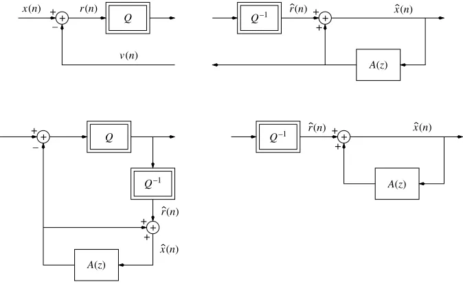
1.3.5. Closed-loop predictive scalar quantization
Let us look at the diagram of the principle of predictive quantization in Figure 1.3. In this configuration, the quantizer requires the transmission at each instantnof the number i(n), the result of the calculation of the prediction error y(n), as well as of another number which is associated with the prediction quantizationv(n)itself. This quantization configuration, known as open-loop quantization configuration, is not realistic because we are not interested in multiplying the information to be encoded, at a constant resolution. The application of a closed-loop quantization is preferred as shown in Figure 1.4 since we can devote all the binary resources available to quantifying the prediction errory(n). The transmission ofv(n)to the receiver is no longer necessary sincev(n)now represents the prediction of the reconstructed signal ˆ
x(n). This prediction can be produced in an identical manner at the transmitter. All that is needed at the transmitter is a copy of the signal processing carried out at the receiver. We can speak of local decoding (at the transmitter) and of distance decoding
+ +
+
Q
+ +
– –
Q–1
Q–1 Q–1
+ +
+
A(z)
A(z)
A(z)
x(n)
x(n)
x(n)
Q
+ +
+ +
+
v(n)
x(n) r(n)
r(n)
r(n)
r(n)
(at the receiver). This method of proceeding has a cost: the prediction is made on the reconstructed signalx(n)ˆ rather than on the original signalx(n). This is not serious as long asx(n)ˆ is a good approximation ofx(n), when the intended compression rate is slightly increased.
We can now turn to the problem of determining the coefficients for the polynomial A(z). The signals to be quantized are not time-invariant and the coefficients must be determined at regular intervals. If the signals can be considered to be locally stationary overN samples, it is enough to determine the coefficients for everyN sample. The calculation is generally made from the signal x(n). We say that the prediction is calculatedforward. Although the information must be transmitted to the decoder, this transmission is possible as it requires a slightly higher rate. We can also calculate the filter coefficients from the signalx(n)ˆ . In this case, we say that the prediction is calculatedbackward. This information does not need to be transmitted. The adaptation can even be made at the arrival of each new samplex(n)ˆ by a gradient algorithm (adaptive method).
Let us compare the details of the advantages and disadvantages of these two methods separately. Forwardprediction uses more reliable data (this is particularly important when the statistical properties of a signal evolve rapidly), but it requires the transmission of side informationand we must wait until the last sample of the current frame before starting the encoding procedure on the contents of the frame. We therefore have a reconstruction delay of at leastN samples. With a backward
prediction, the reconstruction delay can be very short but the prediction is not as good because it is produced from degraded samples. We can also note that, in this case, the encoding is more sensitive to transmission errors. This choice comes down to a function of the application.
Vector Quantization
2.1. Introduction
When the resolution is low, it is natural to group several samples x(n) in a vector x(m) and to find a way to quantize them together. This is known as vector quantization. The resolutionb, the vector dimensionN, and the sizeLof the codebook are related by:
L= 2bN
In this case,bdoes not have to be an integer. The productbN must be an integer or even, more simply,Lmust be an integer. Vector quantization therefore enables the definition of non-integer resolutions. However, this is not the key property of vector quantization: vector quantization allows us to directly take account of the correlation contained in the signal rather than first decorrelating the signal, and then quantizing the decorrelated signal as performed in predictive scalar quantization. Vector quantization would be perfect were it is not for a major flaw: the complexity of processing in terms of the number of multiplications/additions to handle is an exponential function ofN.
2.2. Rationale
Vector quantization is an immediate generalization of scalar quantization. Vector quantization ofN dimensions with sizeLcan be seen as an application ofRN in a finite setCwhich containsL N-dimensional vectors:
The spaceRN is partitioned intoLregions or cells defined by:
Θi={x:Q(x) = ˆxi}
The codebookCcan be compared with a matrix where necessary, andxˆi is the reproduction vector. We can also say thatCrepresents the reproduction alphabet and
ˆ
xi represents the reproduction symbols in accordance with the usual vocabulary for information theory.
Equation [2.1] is a direct generalization of equation [1.1] which uses the probability density function and the Euclidean norm:
σQ2 =
1 N
L
i=1 u∈Θi
||u−ˆxi||2pX(u)du [2.1]
We need to determine the codebook C, that is, the reproduction vectors {xˆ1· · ·ˆxL} while minimizing σ2
Q. This minimization leads us to the identical necessary conditions for optimization that we found for the scalar case:
– Given a codebookC=xˆ1· · ·xˆL, the best partition is that which satisfies:
Θi={x:||x−xˆi
||2≤ ||x−xˆj
||2 ∀j∈ {1· · ·L} }
This is the nearest neighbor rule. This partition is called the Voronoï partition. – Given a partition, the best reproduction vectors are found using the centroid condition. For a quadratic distortion:
ˆ
xi=E{X|X ∈Θi}=
ΘiupX(u)du
ΘipX(u)du
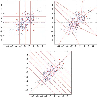
The left-hand chart in Figure 2.1 shows a realizationx(n)of a random process AR(2) which is Gaussian and centered as a function ofn. The right-hand chart is obtained from this realization by creating two-dimensional vectors (N = 2) such thatx(m) = [x(2m)x(2m+ 1)]tand projecting each vectorx(m)in the plane. We obtain a cloud of points which has the tendency to align in proportion along the first diagonal as the first normalized autocovariance coefficient approaches 1.
The graphs in Figure 2.2 show two ways of partitioning the plane. The Voronoï partition corresponds to vector quantization which has been obtained by applying the generalized Lloyd–Max algorithm (see the following section) to the vector case with
20 40 60 80 100 120 140 –10
–5 0 5 10
–10 –8 –6 –4 –2 0 2 4 6 8 10 –10
–8 –6 –4 –2 0 2 4 6 8 10
Figure 2.1.Example of a realization of an AR(2) random process
–8 –6 –4 –2 0 2 4 6 8 –8
–6 –4 –2 0 2 4 6 8
–8 –6 –4 –2 0 2 4 6 8 –8
–6 –4 –2 0 2 4 6 8
Figure 2.2.Comparison of the performance of vector and scalar quantization with a resolution of 2. Vector quantization has L = 16 two-dimensional reproduction vectors. Scalar quantization has L = 4 reproduction values
Figure 2.3 represents a sinusoidal process which is marred by noise. We can see clearly that vector quantization adapts itself much better to the signal characteristics.
–1 –0.5 0 0.5 1
–1 –0.5 0 0.5 1
–1 –0.5 0 0.5 1
–1 –0.5 0 0.5 1
Figure 2.3.Comparison of the performance of vector and scalar quantization for a sinusoidal process marred by noise
A theorem, thanks to Shannon [GRA 90], shows that even for uncorrelated signals, from sources without memory (to use the usual term from information theory), gain is produced through vector quantization. This problem is strongly analogous to that of stacking spheres [SLO 84].
2.3. Optimum codebook generation
In practice, the probability density functionpX(x)is unknown. We use empirical data (training data) for constructing a quantizer by giving each value the same weight. These training data must contain a large number of samples which are representative of the source. To create training data which are characteristic of speech signals, for example, we use several phonetically balanced phrases spoken by several speakers: male, female, young, old, etc.
We give here a summary of the Lloyd–Max algorithm which sets out a method for generating a quantizer. It is an iterative algorithm which successively satisfies the two optimization conditions.
– For all the samples labeled with the same number, a new reproduction vector is calculated as the average of the samples.
– The mean distortion associated with these training data is calculated, and the algorithm ends when the distortion no longer decreases significantly, that is, when the reduction in the mean distortion is less than a given threshold, otherwise the two previous steps are repeated.
The decrease in the mean distortion is ensured; however, it does not always tend toward the global minimum but only reaches a local minimum. In fact, no theorems exist which prove that the mean distortion reaches a local minimum. New algorithms based on simulated annealing, for example, allow improvements (in theory) in quantizer performance.
Initializing the codebook presents a problem. The Linde-Buzo-Gray (LBG) algorithm [LIN 80], as it is known, is generally adopted, which can resolve this problem. The steps are as follows:
– First, a single-vector codebook which minimizes the mean distortion is found. This is the center of gravity of the training data. We write it as xˆ0(b = 0). If the number of vectors in the training data isL′
, the distortion is:
σQ2(b= 0) =
1 L′
1 N
L′−1
m=0
||x(m)||2=σ2X
since the signal is supposedly centered.
– Next, wesplitthis vector into two vectors writtenxˆ0(b= 1)andxˆ1(b= 1)with
ˆ
x0(b = 1) = ˆx0(b = 0)andxˆ1(b = 1) = ˆx0(b = 0) +ǫ. Choosing the vectorǫ
presents a problem. We choose “small” values.
– Knowing thatxˆ0(b= 1)andxˆ1(b= 1), we classify all the vectors in the training data relative to these two vectors (labeling all the vectors 0 or 1), and then calculate the new centers of gravityxˆ0(b = 1)andˆx1(b = 1)of the vectors labeled 0 and 1, respectively.
– The distortion is calculated:
σQ2(b= 1) =
1 L′
1 N
L′−1
m=0
||x(m)−xˆ||2
and this process is iterated as long as the decrease in the distortion is significant. Notice that the decrease is constantly ensured, thanks to the particular choice of initial vectors. In this way, the nearest neighbor rule and the centroid condition are applied a certain number of times to obtain the two reproduction vectors which minimize the mean distortion.
– We split these two vectors afresh into two, and so on.
2.4. Optimum quantizer performance
In the framework of the high-resolution hypothesis, Zador [ZAD 82] showed that the Bennett equation (scalar case),
σ2
which gives the quantization error power as a function of the marginal probability density function of the process and the resolution, can be generalized to the vector case. We find:
wherepX(x)now represents the probability density function andα(N)is a constant which depends only onN. In the Gaussian case:
σ2
As in the case of predictive scalar quantization, we can assess the performance improvement brought about by vector quantization relative to scalar quantization. The vector quantization gainis defined similarly to [1.11] and comprises two terms:
Gv(N) =
The second ratio represents how vector quantization takes account of the correlation between the different vector components. WhenN → ∞, the ratio tends toward the asymptotic prediction gain valueGp(∞)as shown in equation [1.12].
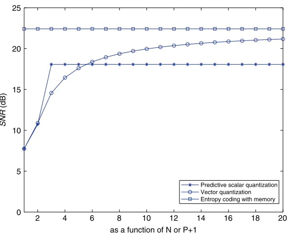
Figure 2.4 shows the signal-to-noise ratio for vector quantization (as a function of
N) and for predictive scalar quantization (as a function ofP+ 1) forb= 2. The limit of the signal-to-noise ratio for vector quantization can be seen whenN tends toward infinity. The signal-to-noise ratio for predictive scalar quantization is:
SNRQSP= 6.02b−4.35 + 10 log10Gp(∞)
when P ≥ 2. The 4.35-dB shift between the two horizontal lines is from the ratio
c(1)/c(∞). Vector quantization offers a wide choice in the selection of the geometric shape of the partition. This explains the gain of 4.35 dB (when N tends toward infinity).
Vector quantization makes direct use of correlation in the signal. Predictive scalar quantization also uses this correlation but only after decorrelating the signal.
2 4 6 8 10 12 14 16 18 20
0 5 10 15 20 25
as a function of N or P+1
SNR
(dB)
Predictive scalar quantization Vector quantization Entropy coding with memory
As soon asN is greater than a relatively low value, vector quantization performs better than predictive scalar quantization. AsNincreases, the performance of vector quantization rapidly approaches the limit for a time-invariant process. It can be shown that no quantizer is capable of producing a signal-to-noise ratio better than this limit. Vector quantization is therefore considered to be the optimum quantization, provided thatN is sufficiently large.
2.5. Using the quantizer
In principle, quantizing a signal involves regrouping the samples of the signal to be compressed into a set ofN-dimensional vectors, applying the nearest neighbor rule to find the vector’s number for encoding and extracting a vector from a table to an address given to supply the reproduction vector for decoding. In practice, a whole series of difficulties may arise, usually due to the processor’s finite calculation power when processing; both encoding and decoding must generally be performed in real time. In fact, the most intensive calculations come from encoding since decoding the processor only needs to look up a vector at a given address in a table.
Let us take the example of telephone-band speech with a resolutionb = 1. We want to perform an encoding at, for example, 8 kbit/s. We must answer the question of how to choose the vector dimensionNand the numberLof vectors which form the codebook. We have just seen that it is in our interests to increaseNbut the size of the codebook increases exponentially sinceL= 2bN. The calculation load (the number of multiplications–accumulations) also increases exponentially withN L =N2bnwith
2bNper sample or2bNf
emultiplications–accumulations per second. We can assume that current signal processors can handle around108multiplications–accumulations
per second. Therefore, we must have:
2bN×8×103≤108
which leads to N ≤ 13 forb = 1. This is too low for at least two reasons. On the one hand, speech signals are too complex to summarize in213 vectors. On the
other hand, the autocorrelation function does not cancel itself out in a few dozen samples. Vector quantization does not require that the components of the vector to be quantized are decorrelated (intraframe correlation) since it adapts correctly to this correlation. However, the vectors themselves must be as decorrelated as possible (interframe decorrelation). WhenN = 13, the interframe correlation is still significant for speech signals.
2.5.1. Tree-structured vector quantization
Take a collection of codebooks, each containing two vectors (binary tree case). In the first stage, we select the nearest neighbor to x(m) in the first codebook. In the second stage, we select the nearest neighbor to x(m)in one or other of the two codebooks depending on the first choice, etc. The calculation cost per sample for a standard codebook is2bN. This reduces to2bN when a binary tree structure is used. The LBG algorithm is well adapted to constructing this codebook since it supplies all the intermediate codebooks (with a little adaptation). Note that the decoder uses only the codebook of size2bN.
2.5.2. Cartesian product vector quantization
A vector is decomposed into several sub-vectors which eventually have different dimensions and a vector quantization is applied individually to each sub-vector. We therefore lose the use of the statistical dependence between the vector components. A method of decomposing the vector so that no dependence exists between the sub-parts is required. The complexity becomes proportional to
iLi, whereLiis the number of vectors in the codebookCi.
2.5.3. Gain-shape vector quantization
This is a special case of the previous case. The idea involves separating the shape characteristics, the spectral content of the vector, and the gain characteristics, the vector energy, into two distinct codebooks. The vector codebook is therefore composed of vectors which are (eventually) normalized. Let us take speech signals as an example. The spectrum content is slightly modified when speech is soft or loud. However, the energy in the signal is strongly amplified. These two types of information are highly decorrelated and therefore justify the use of this method.
2.5.4. Multistage vector quantization
Successive approximations are used in this process. First, a coarse vector quantization is carried out, then a second quantization on the quantization error, etc. as illustrated by Figure 2.5.
2.5.5. Vector quantization by transform
+ +
+ + – –
+ +
+
x(n)
+ +
+ Q1
Q–1 1
Q2
Q–1 2
Q3
Q–1 1
Q–12
Q–13
i 3 (n)
i 1(n)
i (n) 2
x(n)
Figure 2.5.Multistage scalar or vector quantization
not very interesting. To encode signals, a initial transformation is often applied followed by quantization in the transformed domain, but this quantization is usually scalar. An entire chapter is dedicated to this subject. It is sometimes useful to associate a transformation and vector quantization to concentrate information in a lower dimensional vector by neglecting low-energy components. The reduction in complexity that comes about from this truncation can be important. Some classic orthogonal transformations in signal processing include, for example, the discrete Fourier transform and the discrete cosine transform, which has the advantage, in relation to the previous method, of being real-valued.
2.5.6. Algebraic vector quantization
In this method, the codebook is no longer constructed using the Lloyd–Max algorithm. It is independent of the source statistics. The reproduction vectors are regularly distributed in space. This is known as trellis vector quantization. These codebooks are widely used since they reduce the calculation load significantly and they need not be memorized.
2.6. Gain-shape vector quantization
One particular type of vector quantization, known as gain-shape quantization, is widely used, especially for audio signal coding, since this vector quantization can manage the time evolution of the instantaneous power of a sound source conveniently. Rather than minimizing the norm||x−xˆj||relative toj,||x−gˆixˆj
2.6.1. Nearest neighbor rule
Two codebooks are used as shown in Figure 2.6. The first codebookxˆ1· · ·xˆL1
comprises L1 N-dimensional vectors which are possibly normed, and the second codebook
ˆ
g1· · ·ˆgL2 comprisesL2 scalars. Minimizing the squared error relative
to the two indices i and j can be done through an exhaustive search. However, the preferred method to find the minimization is, at the expense of making an approximation, done in two steps. First, the vector in the first codebook which most closely representsxis found. Next, the gain is calculated using a scalar method.
g1...gP
Figure 2.6.Gain-shape vector quantizer
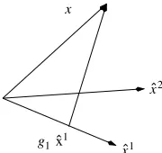
Let us consider the system depicted in Figure 2.7.
g1 x
x1
x1
x2
Figure 2.7.Gain-shape vector quantization
The gain,g(j), is defined so that the vectorg(j) ˆxjis the orthogonal projection of
xonxˆj. This gain is given by:
< x−g(j)ˆxj,xˆj>= 0
g(j) = < x,xˆ
j>
||xˆj||2
where< x, y >is the scalar product of the two vectorsxandy. Since:
by substituting in the value for g(j), the minimization relative to j becomes a
whereφj represents the angle betweenxandxˆj
. The nearest neighbor rule involves therefore, in this case, choosing the vector which is at the lowest angle (to withinπ) toxfrom all the possible vectors.
2.6.2. Lloyd–Max algorithm
We now show how to construct the first codebook, which is characteristic of the shape. We have seen that the Lloyd–Max algorithm is made of two stages. Knowing the training data ofM vectorsx(m)and an initial codebook made ofL1vectorsxˆj, which are assumed to be normalized without losing any generality, we need to find the best partition of M vectors intoL1 classes. Each vector in the training data is labeled by the indexj which maximizes< x(m),xˆj>2. Knowing this partition, the
rest of the codebook can then be determined. From the M(j)vectorsx(m), which are associated with the previous vectorxˆj, the new vectorxˆj which minimizes the meansquared error is calculated:
σQ2(j) =
is maximized with regard toˆxjwhereΓis the empirical covariance matrix:
Γ =
M(j)
m=1
x(m)xt(m)
MaximizingQwithin the constraint||xˆj|| = 1is achieved through the Lagrange multipliers method. The derivative of:
(ˆxj)tΓˆxj
−λ[(ˆxj)txˆj −1]
with respect toxˆjis canceled out. We find:
The parameterλis therefore an eigenvalue of the matrixΓ. By multiplying this equation by(ˆxj)t, we find:
(ˆxj)tΓˆxj =λ(ˆxj)txˆj=λ
Sub-band Transform Coding
3.1. Introduction
Until very recently, a classic distinction was made between transform coding and sub-band coding. In a transform coder, anN-dimensional vector is first determined from the signal. Next, a generally orthogonal or unitary matrix is applied (for example, a matrix constructed from the discrete Fourier transform or the discrete cosine transform), then the coefficients are encoded in the transformed domain. At the receiver, the reverse transform is applied. In a sub-band encoder, the signal is first filtered by a bank of analysis filters, then each sub-band signal is downsampled and the downsamples are encoded separately. At the receiver, each component is decoded, an upsampling and interpolation by a bank of synthesis filters is carried out, then the separate reconstituted signals are added together. These two encoding techniques are equivalent, as will be shown in section 3.2. For further details, refer to the theory of perfect reconstruction filter banks [MAL 92, VAI 90], multi-resolution systems, and wavelet transforms [RIO 93].
We will also see that minimizing the mean squared error (MSE), the criteria with which we are concerned at present, has the effect of making the quantization noise as white as possible. This approach is somewhat theoretical: in practice, the issue is not really aiming at making the quantization noise as low or as white as possible. Rather, we look to constrain the shape of the noise spectrum so that it fits within psychoacoustic or psychovisual constraints. This is known as “perceptual” coding. This question is not addressed in this chapter; it will be broached in Part 2 of the book.
3.2. Equivalence offilter banks and transforms
Consider a bank ofM filters with scalar quantization of sub-band signals as shown in Figure 3.1. Assume that the filters are all finite impulse response filters, causal, with the same number of coefficientsN. The downsampling factor isM′
andb0· · ·bM−1 are the numbers of bits assigned to the quantization of each sub-band signal. When
M′
=M, quantization in the transform domain has the same number of samples as it would have if quantization had been carried out in the time domain. At this point, downsampling iscritical, the filter bank is atmaximum decimation. This is the usual choice in encoding (our assumption is verified as follows).
M +
Figure 3.1.Diagram of a sub-band coding system (with critical downsampling)
from the sub-band signals, theMequations:
can be written in matrix form:
y(m) =
The analysis filter bank is therefore equivalent to a transformationT which is characterized by a rectangular matrixM×Nin which the line vectors are the analysis filter impulse responses. We can also show that a bank of synthesis filters is equivalent to a transformation P which is characterized by a rectangular matrix N ×M in which the reversed column vectors are analysis filter impulse responses. The general condition for perfect reconstruction, the bi-orthogonality condition, is simply that the matrix multiplicationPT results in the identity matrix when N = M (in the trivial case). In the usual case whereN > M (non-trivial case), the bi-orthogonality condition is generalized [VAI 90].
Finding impulse responses hk(n) and fk(n) which satisfy this condition is a
difficult problem. To simplify the problem, we usually1do withmodulatedfilter banks by introducing a strong constraint on hk(n) and fk(n). These impulse responses are obtained from prototype filter impulse responsesh(n)andf(n)via modulation:
hk(n) =h(n)dk(n)andfk(n) =f(n)dk(n)fork= 0· · ·M−1andn= 0· · ·N−1. Note that equation [3.1] becomes:
y(m) =D u(m) with u(m) =h⊗ x(m)
whereD is the modulation matrix and the operation⊗involves multiplying the two vectors component by component. The vectoru(m)is simply the version of the vector
x(m)weighted by the weighting windowh.
dk(n), h(n), and f(n) must be determined. Starting from an ideal low-pass
prototype filter with frequency cut-off1/4M, and constructing from this prototype filter the frequency responseH0(f)· · ·HM−1(f)of theM bank filters as follows:
we can directly deduce the relation between the impulse responses:
hk(n) = 2h(n)cos
2π2k+ 1 4M n
We can find equivalent relations for the synthesis filter bank. In practice, it is impossible to prevent overlapping in the frequency domain as a result of the finite nature of N. Similarly, solutions to the problem of perfect reconstruction do exist. The classic solution is the modified discrete cosine transform (MDCT, TDAC, MLT, etc.), where the matrixDis a cosine matrix with suitable phases:
dk(n) =
!
2 Mcos
"
(2k+ 1)(2n+ 1 +N−M) π 4M
#
fork= 0· · ·M−1andn= 0· · ·N−1.
We can show that the perfect reconstruction condition is written as:
h2(n) +h2(n+M) = 1 for n= 0· · ·M −1
[3.2]
with:
f(n) =h(n) for n= 0· · ·N−1
and this condition is satisfied by:
h(n) =f(n) =sin"(2n+ 1) π 4M
#
This transform is well used (in audio coding).
All that remains for us to do is to determineNandM. This is a delicate question in practice since the transform must satisfy opposing constraints. We generally want good frequency properties (low overlapping in the frequency domain, good frequency resolution) without negatively affecting the time resolution (to handle rapid variations in the instantaneous signal power). This question will be addressed in the second part of the book.
3.3. Bit allocation
3.3.1. Defining the problem
TheM componentsyk(m)of the vectory(m) = Tx(m)can be interpreted as the realization ofM time-invariant random processesYk(m)with powerσ2Yk. The
quantization error powers are written asσ2
Q0· · ·σ 2
QM−1. By admitting that the perfect reconstruction condition involves conserving the power as in the case of an orthogonal or unitary transform, we deduce that the reconstruction error power (which is of interest to the user):
σ2 ¯
Q=E{|X(n)−Xˆ(n)|
2}= 1
NE{||X(m)−Xˆ(m)||
is equal to the arithmetic mean of the quantization error powers of the different components (errors introduced locally by the quantizers):
σ2
The first problem that we examine is as follows. We apply an ordinary transform T. We haveM bits at our disposal to scalar quantize theM coefficients, theM sub-band signals. We need to find the optimum way of distributing thebMbinary resources available. This requires, therefore, that we determine the vectorb = [b0· · ·bM−1]t while minimizingσ2
Qwithin the constraint: M−1
k=0
bk≤bM
3.3.2. Optimum bit allocation
In the framework of the high-resolution hypothesis, we can express σ2
Qk as a
function of σ2
Yk andbk by applying [1.5]. Recall that the expression underlines the
fact thatσ2
whereck(1) is a constant which depends only on the marginal probability density function ofYk(m). The repercussions of the hypothesis of Gaussian form on the sub-band signals are that all the constantsck(1)are equal. This common constant is known
asc(1).
Let us show that the optimum bit allocation which minimizes:
σ2
within the constraintM−1
k=0 bk ≤bMis given by:
wherebis the mean number of bits per component and:
is the geometric mean of the powers.
In effect, we know that as long as we haveM positive real numbers, the arithmetic mean is greater than or equal to the geometric mean and that this equivalence occurs when theMnumbers are equal as follows:
1
, this relation becomes:
1
The optimum value is achieved when all the intermediate terms in the sum are equal. In this case, the inequality becomes an equality. Whatever the value of
kis, we have:
Hence, we find equation [3.5].
Equation [3.6] has an interesting interpretation. It means that the optimum scalar quantization of each random variableYk(m)gives rise to the same MSE. We therefore arrive at the following important conclusion: everything happened as though we were seeking to make the reconstruction error as close as possible to a full-band white noise.
The quantization error power can be written as:
![Figure 1.1. (a) The signal before quantization and the partition of the range[−A, +A] and (b) the set of reproduction values, reconstructed signal, andquantization error](https://thumb-ap.123doks.com/thumbv2/123dok/1319495.2011403/15.595.131.466.344.513/figure-signal-quantization-partition-reproduction-values-reconstructed-andquantization.webp)