Full Terms & Conditions of access and use can be found at
http://www.tandfonline.com/action/journalInformation?journalCode=ubes20
Download by: [Universitas Maritim Raja Ali Haji] Date: 12 January 2016, At: 00:13
Journal of Business & Economic Statistics
ISSN: 0735-0015 (Print) 1537-2707 (Online) Journal homepage: http://www.tandfonline.com/loi/ubes20
Inference in Nearly Nonstationary SVAR Models
With Long-Run Identifying Restrictions
Nikolay Gospodinov
To cite this article: Nikolay Gospodinov (2010) Inference in Nearly Nonstationary SVAR Models With Long-Run Identifying Restrictions, Journal of Business & Economic Statistics, 28:1, 1-12, DOI: 10.1198/jbes.2009.08116
To link to this article: http://dx.doi.org/10.1198/jbes.2009.08116
Published online: 01 Jan 2012.
Submit your article to this journal
Article views: 152
View related articles
Inference in Nearly Nonstationary SVAR Models
With Long-Run Identifying Restrictions
Nikolay G
OSPODINOVDepartment of Economics, Concordia University, 1455 de Maisonneuve Blvd. West, Montreal, Quebec, H3G 1M8 Canada (nikolay.gospodinov@concordia.ca)
This paper considers inference for impulse responses in models with highly persistent variables. We show that the impulse responses of interest are not consistently estimable under the long-run identification scheme when the strongly dependent process is parameterized as local to unity. We employ the instru-mental variable framework to argue that the inconsistency and the large sampling uncertainty associated with the impulse responses arise from a weak instrument problem. Furthermore, the structure of the model is used to impose additional statistical restrictions that are combined with the economic long-run, identi-fying constraints to obtain an improved estimator.
KEY WORDS: Impulse response analysis; Local-to-unity asymptotics; Long-run restrictions; Persis-tence.
1. INTRODUCTION
Imposing long-run identifying restrictions in structural vec-tor auvec-toregressive (SVAR) models has become a popular method for conducting inference on impulse response functions (IRFs) and recovering structural shocks. In a seminal paper, Blanchard and Quah (1989) use long-run identifying restric-tions to study the contribution of supply and demand shocks to business cycle fluctuations. Over the last two decades, the long-run identifying scheme has been applied extensively in the empirical macroeconomic and international finance liter-ature. More recently, this framework has been used by Gali (1999), Christiano, Eichenbaum, and Vigfusson (2006), Fran-cis and Ramey (2005), and Pesavento and Rossi (2005), among others, to empirically evaluate the prediction of real business cycle (RBC) models that technology shocks have a positive ef-fect on hours worked.
Despite its widespread popularity and intuitive appeal, the long-run identifying scheme has been criticized on several grounds. Cooley and Dwyer (1998) question Blanchard and Quah’s (1989) theoretical framework, identifying assumptions and statistical methodology. Faust and Leeper (1997) raise some concerns that long-run restrictions may deliver very unre-liable impulse response estimates in finite samples. Chari, Ke-hoe, and McGrattan (2005) argue that the SVAR-based infer-ence procedures can be misleading and cannot serve as a useful guide to developing and evaluating dynamic economic mod-els. In response to the Chari, Kehoe, and McGrattan (2005) cri-tique, Christiano, Eichenbaum, and Vigfusson (2006) provide convincing evidence that SVARs perform very well in practi-cally relevant cases but they also find that the sampling uncer-tainty associated with the IRFs based on SVAR with long-run identifying restrictions is fairly large and the estimated wide confidence bands are not particularly useful in distinguishing between competing economic theories.
This paper studies the statistical properties of the IRF esti-mator in the context of the technology shock example where labor productivity is assumed to have an exact unit root and hours worked are modeled as a near-integrated process. The paper develops the asymptotic distribution theory for the struc-tural parameters in a SVAR model with long-run restrictions
and provides formal results that shed light on the large sam-pling uncertainty of the conventional IRF estimator. Using an instrumental variable framework, we show that the high persis-tence in hours worked gives rise to a weak instrument prob-lem which in turn leads to a highly nonstandard limiting the-ory. The asymptotic representations have the form of a ratio of random variables which produces distributions with heavy tails. Moreover, we demonstrate that the IRF estimator in the adopted setup is inconsistent and its sampling uncertainty can-not be reduced as the sample size increases. Finally, we propose an alternative method that combines economic and statistical restrictions and delivers a consistent and asymptotically normal IRF estimator with a substantially smaller sampling variation and bias. The statistical restriction is derived from the particu-lar structure of the matrix containing the particu-largest roots of the sys-tem. This, in combination with the long-run identifying scheme, places restrictions on the structural parameters that are not con-sistently estimable under the traditional approach and removes the source of the inconsistency for the structural IRF. From a practical point of view, the restricted IRF estimator is easy to compute and is valid over both the stationary and nonstationary regions of the parameter space.
The rest of the paper is organized as follows. Section2 intro-duces the model and its different reparameterizations. Section3 derives the main asymptotic results and proposes a method that utilizes the structure of the model to combine economic and sta-tistical restrictions for improved inference. Section4 provides some simulation results and Section5concludes.
2. MODEL AND ASSUMPTIONS
Consider the reduced form of a bivariate vector autoregres-sive processyt=(lt,ht)′of orderp+1
(L)(I−L)yt=ut, (1)
© 2010American Statistical Association Journal of Business & Economic Statistics
January 2010, Vol. 28, No. 1 DOI:10.1198/jbes.2009.08116
1
where the matrixcontains the largest roots of the system and
. The presence of de-terministic components in (1) does not affect directly the shape of the impulse response function but it has an effect on the dis-tribution of some of the model parameters. Some discussion on how the limiting results should be modified in the presence of deterministic components is provided later in the paper.
The notation is chosen to be consistent with our leading ex-ample that studies the response of hours worked to a shock in technology. The econometric model used to address this ques-tion is built upon several model assumpques-tions and stylized empir-ical facts. One assumption that appears to be least controversial is that the first variable (labor productivity or output) is an ex-act unit root process. This is consistent with the standard RBC model that imposes a unit root on technology. In principle, one could further generalize the model by allowing for the possi-bility that labor productivity is a strongly dependent stationary variable around a deterministic trend. In this case, the long-run restriction that nontechnology shocks have no permanent effect on labor productivity does not achieve identification. One way to identify the structural parameters is to assume that only tech-nology shocks have a permanent effect on labor productivity at lead times that are of the same order as the sample size (Wright 1996).
In the recent literature, the debate on the effect of technology on hours worked has been largely driven by the econometric specification of hours worked. In particular, Gali (1999) and Francis and Ramey (2005) include hours worked in first differ-ences and find that the initial response of hours to a positive shock in technology is negative. Christiano, Eichenbaum, and Vigfusson (2003) carefully analyze the time series properties of hours worked and conclude that the most appropriate speci-fication for this variable is in levels. In this case, the estimated impulse response function is in agreement with the RBC model. As a result, we model labor productivity as a unit root process and allow hours worked to evolve as a highly persistent process whose largest AR root lies near the boundary of nonstationarity but the two processes are not cointegrated.
More formally, we parameterizeas T =
1 0 parameterization reflects the uncertainty about the magnitude of the largest root of hours worked and was recently used by Pe-savento and Rossi (2005,2006). The local-to-unity reparame-terization is an artificial statistical device that proves useful for obtaining more accurate finite-sample approximations when the largest AR root is believed to be close to unity. The off-diagonal elements ofT are set to 0 to rule out the case that any of the
two processes is (near-)I(2)(Elliott1998; Phillips1988). The possibility of nonzero off-diagonal elements is discussed later in the paper. For notational convenience, the dependence of
onT is subsequently suppressed. Extensions to higher dimen-sional SVARs will depend on the structure of the problem. If there is only one local-to-unity variable and the remaining vari-ables are weakly dependent, the generalization of the model is straightforward. If the local-to-unity processes in the system are more than one, the model needs to be modified depending on whether these processes are cointegrated or not. We do not con-sider these more general specifications in this paper.
Below we list the conditions that are needed for deriving the limiting results in the next section.
Assumption 1. Assume that:
(a) The determinantal equation|(z)| =0 has roots outside the unit circle and(z)−1is one-summable.
(b) ut is a two-dimensional martingale difference sequence
withE(utu′t|ut−1,ut−2, . . .)= and suptEut2+ξ for
someξ >0, whereis positive definite. (c) y0,y−1, . . . ,y−pareOp(1).
is a stationary linear process. To preserve the usual interpre-tation of the impulse response functions, one may need to strengthen part (b) of Assumption1by assuming thatut is iid
withEut2+ξ for some ξ >0.The initial conditions are
as-sumed fixed and, without loss of generality, can be set equal to zero. Finally, the largest roots of the system are assumed to be one and local to unity and the two processes are not cointe-grated.
It proves useful to express model (1) in the Blanchard-Quah framework by imposing the exact unit root on productivity so that△lt is a stationary process. In this case, letyt=(△lt,ht)′
and A(L)=(L)1 0 0 1−(1+c/T)L
. Then, the reduced form VAR model is given by
A(L)yt=ut,
(2)
yt=A1yt−1+ · · · +Ap+1yt−p−1+ut.
Premultiplying both sides of (2) by the matrix B0 = 1 −b(0)
12
−b(210) 1
yields the structural VAR model
B(L)yt=εt,
where B(L)=B0A(L) and εt =B0ut denote the structural
shocks(εtz, εdt)′ which, following the typical practice, are
as-sumed to be orthogonal with variancesσ12andσ22. The long-run identifying restriction that the nontechnology shocksεtdhave no long-run effect on labor productivity imposes a lower triangu-lar structure on the moving average matrixA(1)−1B−01. Hence, under this identifying restriction, the matrix of long-run mul-tipliers in the structural model,B(1)=B0A(1),is also lower
triangular.
3. INFERENCE IN MODELS WITH A HIGHLY PERSISTENT VARIABLE AND LONG–RUN
IDENTIFYING RESTRICTIONS
3.1 Pitfalls in Imposing Long-Run Identifying Restrictions
It is convenient to rewrite the reduced model (2) in the Dickey–Fuller form (Stock1991)
yt=A∗(1)yt−1+
p
i=1
A∗∗i △yt−i+ut, (3)
whereA(L)=(L)(I−L),A∗(L)=L−1(I−A(L)),A∗(1)=
After imposing the restriction that the long-run multiplier of hours worked is zero (which is equivalent to assuming that the nontechnology shocks have no long-run effect on labor produc-tivity), the structural model reduces to
△lt=b(120)△ht+
Since our interest lies in the structural parametersb(120) and b(210), whose statistical properties determine the limiting behav-ior of the impulse response function, we rewrite the model (up toop(1)terms) as
△lt=b(120)△ht+εzt, (6)
△ht=b(210)△lt+b∗22ht−1+εdt, (7)
where△lt and△ht are defined as residuals from projections
on the predetermined variables(△lt−1, . . . ,△lt−p,△ht−1, . . . ,
△ht−p)that enter both the structural and reduced form
mod-els. The reduced form VAR in (4) can be rewritten in a similar fashion.
First, we consider the instrumental variable (IV) estimation of the unknown parameter b(120) using ht−1 as an instrument.
The IV estimation of SVAR models that we employ here has been considered before by Christiano, Eichenbaum, and Vig-fusson (2003), Hausman, Newey, and Taylor (1987), Pagan and Robertson (1998), Fry and Pagan (2005), Sarte (1997), Shapiro and Watson (1988), and Watson (1994,2006), among others. The relationship between the endogenous variable and the in-strument is given by the second equation of the reduced VAR model
△ht=ψ22(1)
c
Tht−1+u2,t. (8) Note that the local-to-unity parameterization automatically translates into a local-to-zero correlation between the endoge-nous variable and the instrument. This bears some similarities
to Staiger and Stock’s (1997) analytical framework but here the correlation between the endogenous regressor and the instru-ment shrinks to zero at rateTdue to the (near-) nonstationarity of the instrument (see also Hahn and Kuersteiner2002).
After substituting (6) and (8) in the IV estimator b(120) =
The following theorem presents the limiting theory for the IV estimator ofb(120).
Theorem 1. Under the model assumptions,
b(120)−b(120)⇒ σ1
where V1(r) and V2(r) are independent standard Brownian motions, Jc(r)=exp(cr)
r
0exp(−cs)dV2(s) is an Ornstein–
Uhlenbeck process, ω22 is the lower right element of the long-run covariance matrix =(1)−1(1)−1′ of(L)ut
and ρ is the long-run correlation between εtz and (1−(1+
T−1c)L)ht.
For the proof see theAppendix.
The result in Theorem1shows that the IV estimator ofb(120) is inconsistent. The cause of the inconsistency is thatht−1is a
weak instrument in a sense that it provides very little informa-tion about the endogenous variable△ht. This in turn arises from
the highly persistent nature of the processhtwhich in this paper
is modeled as local to unity. Furthermore, the limiting distrib-ution ofb(120)−b(120) is nonstandard. First, the numerator of the limiting representation is a mixture of a Gaussian random vari-able and a functional of an Ornstein–Uhlenbeck process where the weights are determined by the correlation between the first structural shock and the reduced form errors from the second equation. Second, it is a ratio of two random variables since the denominator is also a random variable that involves functionals of the Ornstein–Uhlenbeck process.
It is instructive to consider the situation whenht approaches
an exact unit root process (c→0). In this case, the distribution ofb(120)−b12(0)has a limit(σ1/ω2)[ρ+ 1−ρ2(1
0V2(s)dV1(s)/ 1
0V2(s)dV2(s))](see also Christiano, Eichenbaum, and
Vig-fusson2003). Furthermore, ifρ→1, the limiting distribution ofb(120)−b(120) approaches a point probability mass at the
con-Now consider the estimation of the parameters in equa-tion (7). Since, by construction,εtz andεtd are orthogonal, we
is derived in the following theorem.
Theorem 2. Under the model assumptions,
are population covariances, δ2 is the squared correlation be-tweenεtdandu2,tandξ ∼N(0,1).
For the proof see theAppendix.
Theorem2establishes that the IV estimator ofb(210) is incon-sistent and its limiting distribution is a function of the limit-ing distribution ofb(120). Note thatb(210) can be obtained equiv-resembles the form of its limiting distribution in Theorem2but it is only in terms of the reduced form shocks. The parame-ter on the persistent variable can be consistently estimated and its asymptotic distribution is a mixture of a Dickey–Fuller and standard normal random variables.
Given the results in Theorems1 and2, we now study the limiting behavior of the impulse response function. Letθhz(l)= ∂ht+l/∂εzt denote the impulse response of hours worked at time
t+lto a one unit shock in technology at timet. In general, the IRF is a complicated nonlinear function of the model parame-ters. Here, we follow Pesavento and Rossi (2006) and approxi-mate the IRF of hours worked asθhz(l)≈ [l(1)−1B−01]21or
Theorem 3. Under the model assumptions,
θhz(l)−θhz(l)=Op(1).
For the proof see theAppendix.
Theorem 3 shows that imposing long-run restrictions in a model with a local-to-unity variable produces inconsistent esti-mators of the impulse response functions. We give this result an instrumental variable interpretation. In particular, the inconsis-tency of the IRF estimators is driven by the presence of a weak instrument. Once we parameterize the second variable (hours worked in our example) as local to unity, the correlation be-tween the instrument and the endogenous variable shrinks to zero at rateT. More specifically, the weak instrument problem in our setup arises from the estimation of b(120) and the incon-sistency of this parameter contaminates the estimation ofb(210) andθhz(l). In the next section of the paper, we argue that impos-ing some a priori statistical restrictions on the parameterb(120) may solve the inconsistency problem for the IRF. In principle, we could combine the results from Theorems1and2to obtain
the asymptotic distribution ofθhz(l)but the resulting distribution is highly nonstandard and nonpivotal and is of limited practical relevance.
Several additional remarks on the results in Theorems1,2, and 3 are in order. Christiano, Eichenbaum, and Vigfusson (2003) and Watson (2006) discuss the weak instrument issue in the technology shock example. Theorems1,2, and3formalize these results and derive the limiting properties of the estima-tors. It is interesting to see how this type of weak identification, driven by the near-nonstationarity of hours worked, affects the procedure by Stock and Yogo (2005) for detecting weak instru-ments. Cooley and Dwyer (1998) and Sarte (1997) also discuss the possibility of weak instruments in SVARs but it is related to the possibly weak correlation betweenεtzand△ltin the
sec-ond equation of our SVAR model. In a different context, Hahn, Hausman, and Kuersteiner (2007) and Han and Phillips (2007) study the weak identification problem that arises from instru-menting the first difference of a highly persistent variable with its lagged level for dynamic panel data models. They provide some suggestions for choosing better instruments that could po-tentially be applied in our framework as well. Finally, in the presence of deterministic components, the asymptotic distrib-utions in Theorems1and2have to be modified by replacing Jc(r) with its demeaned version J∗c(r)=Jc(r)−
1
0 Jc(s)ds,
if the equation for hours worked includes only a constant, or with its detrended versionJc∗∗(r)=Jc(r)−
1
0(4−6s)Jc(s)ds−
r01(12s−6)Jc(s)ds, if hours worked are modeled as a process
with a linear trend.
3.2 Improved Inference by Combining Economic and Statistical Restrictions
Consider the matrix of long-run multipliers in the SVAR foryt
and recall that restricting nontechnology shocks to have no per-manent effect on labor productivity renders matrixB(1)lower triangular.
It is easy to see that forc<0, imposing this long-run re-striction onB(1)constrains the parameters of B0; in
particu-lar,b(120)=ψ12(1)/ψ22(1).In the first-order SVAR model, this
restriction is reduced to b(120)=0. Levtchenkova, Pagan, and Robertson (1998, p. 513) discuss the relationship betweenB0, A(1) and B(1) but do not consider its implications for im-pulse response analysis. Whenc=0, the parameters ofB0are
not directly identifiable from the above representation but the model can be rewritten so that both variables are first differ-enced and the long-run identifying restriction is defined for the cumulative responses of the differenced variables. In this case, it is straightforward to show that the same restriction,b(120)=
ψ12(1)/ψ22(1), renders the moving average structural matrix of
(△lt,△ht)lower triangular. In what follows, we refer to the IRF
estimator that imposes the restrictionb(120)=ψ12(1)/ψ22(1)as restricted estimator and to the conventional IRF estimator ana-lyzed in the previous section as unrestricted estimator.
There are two ways to gain intuition about the differences between the unrestricted and restricted estimators. While both estimators impose the same long-run economic restriction, the conventional unrestricted approach uses separate estimates for the reduced form parameters and the components of the struc-tural model. In contrast, the restricted method estimates the structural parameters by explicitly imposing the one-to-one re-lationship between the reduced and structural forms implied by the long-run economic theory and the statistical model. The dif-ferences between the unrestricted and restricted estimators are even more obvious in the IV framework where the conventional estimator ofb(120) is obtained in an unrestricted manner using a weak instrument whereas the restricted estimator gets around the weak instrument problem by constraining the value ofb(120) to a function of reduced form parameters. The IV framework also helps us infer that as the second variable moves away from the boundary of nonstationarity, the weak instrument problem is alleviated and the differences between the two estimators tend to become smaller and eventually disappear.
It is important to emphasize that the restricted estimator uti-lizes the statistical structure of the model and its validity de-pends crucially on the assumed form of matrix. Pesavento and Rossi (2005) also impose diagonality onto study the ef-fect of technology shocks on hours worked although they do not fully explore its effect on the relationship between the reduced and structural parameters. As we argued above, the zero diago-nal elements of matrixrule out near-I(2) behavior in the vari-ables of interest. In Section3.3we relax the diagonal structure ofand allow for a nonzero (but asymptotically dissipating) upper off-diagonal element that could give rise to a small low frequency component in labor productivity growth which is not readily detectable by examining its dynamics. This generaliza-tion leads to a slight modificageneraliza-tion in the relageneraliza-tion betweenb(120) and the reduced form parameters and the subsequent analysis can be easily adapted to this situation.
The main advantage of explicitly imposing the restric-tion b(120) =ψ12(1)/ψ22(1) is that the source of the inconsis-tency of the IRF estimator is removed. In practice,b(120) =
ψ12(1)/ψ22(1), where ψ12( 1) andψ22( 1) are consistent esti-mators of ψ12(1)and ψ22(1) from the reduced form model.
The estimation of the remaining structural parameters and im-pulse responses is performed as before. The next theorem es-tablishes the limiting distributions of the structural parameters and the impulse response functions in this case.
Theorem 4. Let ψ =(ψ12(1), ψ22(1))′, f(ψ) =ψ12(1)/ orem 2, and γ2 and ϕ2 denote the asymptotic variances of
√
T(b(210)−b(210))and√T(θhz(l)−θhz(l))that are functions of the parameters of the model.
For the proof see theAppendix.
Theorem4reveals that after imposing the restrictionb(120)=
ψ12(1)/ψ22(1),the IV estimator ofb(210)is
√
T-consistent. Fur-thermore, if the lead time is considered fixed, the IRF is also
√
T-consistent. This is due to the fact that iflis fixed, the sam-pling uncertainty associated with the estimation of the largest root in the system vanishes asymptotically asl/Tapproaches 0. In contrast, when the lead time is assumed to be a fraction of the sample size, the parameter estimation uncertainty is preserved and the effect of the estimation error does not vanish asT→ ∞ which renders the IRF estimator inconsistent (Phillips1998). In this case, one could use the method proposed by Pesavento and Rossi (2006). Since in the technology shock example the inter-est typically lies in inter-estimating impulse responses at short and medium horizons, we do not consider explicitly the long hori-zon case.
For the first-order SVAR model, (L)=I and b(120) =0. This simplifies considerably the limiting representations in Theorem 4; in particular, both √T(σ1/σ2)(b(210) −b
Several other features of the results in Theorem 4 deserve closer attention. First, the asymptotic normality of the struc-tural parameters and the IRF may seem somewhat surprising given the presence of a nearly integrated variable in the model. However, the restricted IV estimator turns out to be numeri-cally equivalent to the conventional OLS estimator on the quasi-differenced variables(1−L)ltand(1−(1+T−1c)L)ht. The
lat-ter implicitly imposes zero restrictions on the diagonal elements ofand the transformed stationary variables drive the asymp-totic normality of the IRF estimator. Also, the sampling uncer-tainty of the largest root ofht is assumed to vanish
asymptoti-cally asT→ ∞and does not enter the limiting distribution of the IRF. As mentioned above, this is not the case whenlgrows at the same rate as the sample size and the localizing constantc enters explicitly the asymptotic distribution ofθhz(l).
Second, the suggested procedure places restrictions on both impact and long-run multiplier matrices but it has some impor-tant conceptual differences with the standard short-run iden-tification scheme. While the standard short-run ideniden-tification scheme is typically criticized for adopting arbitrary time con-ventions and lack of robustness, our restriction onb(120)arises as a by-product from jointly restricting the long-run economic and statistical dynamics of the system. If either of these long-run restrictions is not imposed, the contemporaneous matrix in the structural form cannot be constrained.
The practical implementation of the restricted estimation of the structural parameters and IRFs is computationally straight-forward. First, we estimate the parameters of (1) from the Dickey–Fuller form of the reduced VAR in (1) (Stock1991). Alternatively,(L)can be estimated from a VAR in quasi dif-ferences(I−L)yt,where is a preliminary consistent
es-timate of (Pesavento and Rossi2005). Next, we setb(120)=
ψ12(1)/ψ22(1)and estimate the remaining structural parame-ters by IV. Finally, the estimated structural parameparame-ters are used to compute the IRFs to different structural shocks.
3.3 Extensions
In principle, it is possible to generalize the form of by allowing the upper right element of this matrix to depend on the proximity of the largest root of hours worked to one. More specifically, letT =
1 πc/T 0 1+c/T
for some constantπ. In this case, if hours worked have an exact unit root, is diagonal; otherwise, the upper right element of is nonzero and is al-lowed to increase as the root of hours worked moves away from the boundary of nonstationarity without inducing an asymptotic I(2) behavior inlt.
First, note that this extension does not affect the analysis in Section 3.1as the process for ht, which is the source of the
weak instrument problem, is unchanged. Second, this general-ization leads to a simple modification of the restriction ofb(120) with respect to the reduced form parameters in(1)which is now given byb(120)= [π ψ11(1)+ψ12(1)]/[π ψ21(1)+ψ22(1)].
Ifπ is known, an IRF estimator based on this restriction can be constructed as discussed in Section 3.2. Also, this frame-work appears to be more appropriate to study the technology shock example and reconcile the large quantitative and quali-tative differences in the estimated effect of technology shocks on hours worked from the levels and differenced specifications (Gospodinov, Maynard, and Pesavento2008).
4. SIMULATION EXPERIMENT
In this section, we conduct a small Monte Carlo experiment to illustrate the numerical properties of the methods discussed in the paper. The data are generated from the VAR model
(L)
with parameter values that are calibrated to match the empirical shape of the IRF of hours worked to a positive technology shock. To examine the sensitivity of the methods to the persistence ofht and the sample size, we use
c= −10 and 0, andT=250 and 1,000. The estimation of all models is performed on the demeaned△lt andhtwith 10,000
Monte Carlo replications.
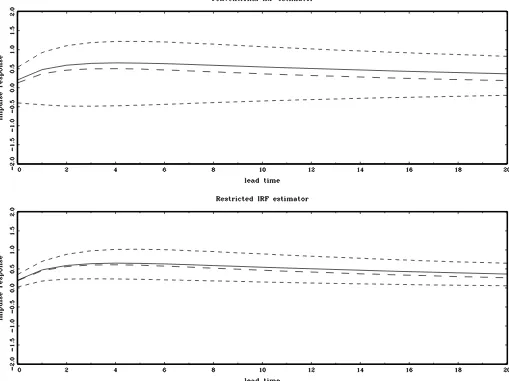
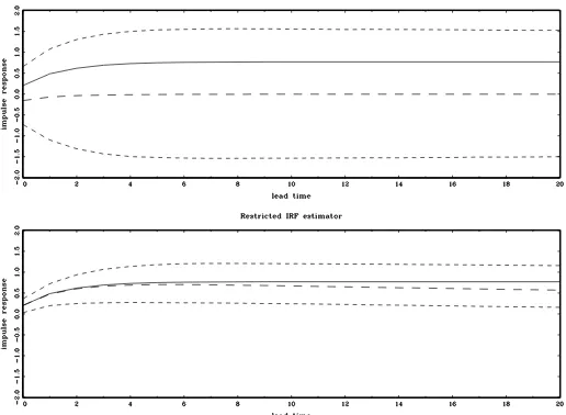
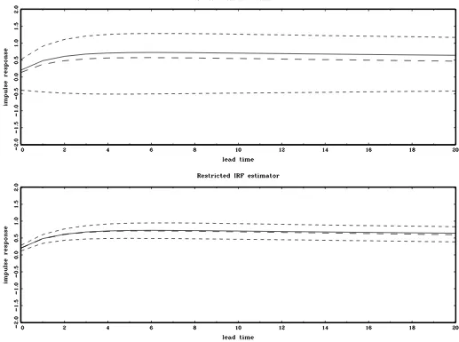
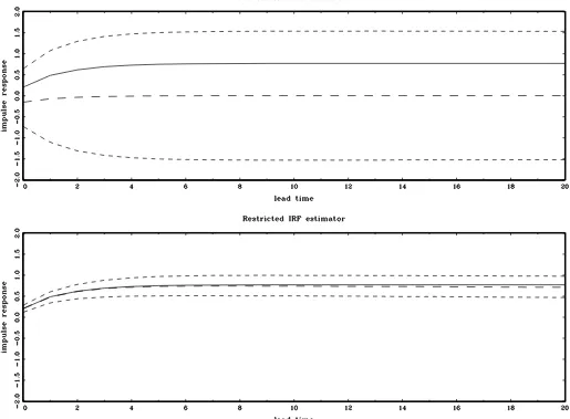
Figures1,2,3, and4plot the true impulse response func-tions, median estimates, and 95% Monte Carlo confidence bands of the IRFs. The upper panel in each figure presents the results for the conventional unrestricted estimator and the lower panel contains the restricted IRFs obtained by imposing b(120)=ψ12(1)/ψ22(1), whereψ12(1)andψ22(1)denote the
es-timated values of ψ12(1)and ψ22(1)from the reduced form
VAR.
The results indicate that imposing the additional restric-tion b(120)=ψ12(1)/ψ22(1) leads to a substantial reduction of
the sampling uncertainty of the restricted IRF estimator com-pared to its unrestricted counterpart. The difference between the sampling uncertainty of the conventional and restricted es-timators becomes larger as the largest root of ht approaches
unity. Also, the conventional IRF estimator is characterized by a large median bias that tends to increase with the degree of
persistence. The large bias of the unrestricted estimator is con-sistent with the results of Christiano, Eichenbaum, and Vig-fusson (2006), obtained from some specifications of the RBC model. At the same time, Christiano, Eichenbaum, and Vig-fusson (2006) also report results from different parameteriza-tions of the RBC model (with a different ratio of variances of the shocks) in which the IRF estimates do not display signifi-cant bias. As in Christiano, Eichenbaum, and Vigfusson (2006), we found that the absolute magnitude of the bias and sampling uncertainty of the IRFs depends on the covariance matrix
although the relative patterns of sampling behavior of the unre-stricted and reunre-stricted estimators remain qualitatively the same. Also, Christiano, Eichenbaum, and Vigfusson (2006) propose a zero-frequency spectral density estimator for bias reduction when a finite-order VAR is fitted to data that are generated from an infinite dimensional VAR or VARMA models. In this paper, we only deal with VAR models of known finite order although the results can be extended to possibly infinite dimensional vec-tor linear process by allowing the lag order of the fitted VAR to increase at a certain rate with the sample size.
Unlike the unrestricted estimator, the bias of the restricted estimator is very small and appears to be less sensitive to the localizing constantcthat governs the persistence of the process. When the sample size is increased to 1,000, the bias of the restricted IRF estimator is negligible and its sampling uncer-tainty is further reduced. In contrast, the sampling unceruncer-tainty of the conventional estimator does not change as the sample size grows which numerically illustrates the inconsistency of this IRF estimator established theoretically in Section3.1.
5. CONCLUDING REMARKS
This paper makes two contributions to the literature on im-pulse response inference. First, it discusses some pitfalls in the inference on impulse response functions based on long-run identifying restrictions. In particular, it provides formal results for the inconsistency of the IRF estimator in a SVAR model when one of the processes is local to unity. The source of the inconsistency is the weak correlation that shrinks to zero at rate T, between the contemporaneous change of the local-to-unity process (endogenous variable) and its lagged level which serves as an instrument in the adopted IV framework. Further-more, we argue that this source of inconsistency can be removed by imposing restrictions on the parameter of the endogenous variable. This is achieved by combining long-run economic re-strictions with additional statistical constraints on the reduced-form VAR matrix of largest roots. We show that this restricted approach delivers a consistent and asymptotically normally dis-tributed IRF estimator. It should be emphasized that the local-to-unity device is used only to approximate better the behavior of the structural parameters and IRFs in the presence of a highly persistent variable and we expect that the practical relevance of the results extend beyond the framework adopted in this paper. The appealing statistical properties of the restricted estimator along with its excellent numerical performance and easy
Figure 1. True impulse response (solid line), Monte Carlo median IRF estimate (long dashes), and 95% Monte Carlo confidence bands (short dashes) computed using simulated data withc= −10 andT=250. The conventional (unrestricted) IRF is obtained from the standard long-run identification scheme and the restricted IRF is obtained by combining long-run economic and statistical restrictions as described in the text.
plementation make the proposed procedure very attractive for applied work.
APPENDIX: MATHEMATICAL PROOFS
A.1 Proof of Theorem1
Let ⇒ signify weak convergence and D[0,1] denote the space of real valued functions defined on the interval [0,1]
that are right-continuous at each point in [0,1] and have finite left limits. Since the assumptions of the model sat-isfy the conditions for the functional central limit theorem (Phillips1988),
1
√
T
[Tr]
t=1
et⇒1/2B(r),
where et =(L)−1ut, =(1)−1(1)−1′ is the
long-run variance–covariance matrix, andB(r)=(B1(r),B2(r))′ is
a vector of two independent standard Brownian motions on D[0,1]. Then, it follows that
T−1/2h[Tr]⇒ω22Jc(r),
whereω22 is the lower right element of matrixandJc(r)=
exp(cr)0rexp(−cs)dB2(s)is an Ornstein–Uhlenbeck process.
Also,
T−1/2
[Tr]
t=1
εzt,T−1/2
[Tr]
t=1
(1−φL)ht
⇒(W1(r),B2(r)),
whereφ=1+T−1c, {W1(r),B2(r):r∈ [0,1]} is a bivariate
Brownian motion in D[0,1] ×D[0,1]with covariance matrix
Ŵ=r σ12 ρσ1ω2 ρσ1ω2 ω22
andρ is the long-run correlation coeffi-cient between(1−φL)htandεtz.
Equivalently, if we letV2(r)=B2(r),we have
1
√
T
[Tr]
t=1
(1−φL)ht
εzt
⇒
ω2
2V2(r)
σ12(ρV2(r)+ 1−ρ2V1(r))
,
Figure 2. True impulse response (solid line), Monte Carlo median IRF estimate (long dashes), and 95% Monte Carlo confidence bands (short dashes) computed using simulated data withc=0 andT=250. The conventional (unrestricted) IRF is obtained from the standard long-run identification scheme and the restricted IRF is obtained by combining long-run economic and statistical restrictions as described in the text.
whereV1(r)andV2(r)are two independent standard Brownian motions.
By the continuous mapping theorem, 1/TTt=2ht−1u2,t⇒
ω2201Jc(s)dV2(s), (c/T2)Tt=2h2t−1 ⇒ ω 2 2c
1
0Jc(s)2ds, 1/
TTt=2ht−1εzt ⇒ σ1ω2(ρ 1
0Jc(s)dV2(s) + 1−ρ2 × 1
0Jc(s)dV1(s)). Combining these results gives
b(120)−b(120)⇒σ1
ω2
ρ01Jc(s)dV2(s)+ 1−ρ2 1
0Jc(s)dV1(s)
c01Jc(s)2ds+01Jc(s)dV2(s)
.
A.2 Proof of Theorem2
Rewrite the IV estimator forβ=(b21(0),b(221))as
β−β=
1 T
T
t=2 ztx′t
−1
1 T
T
t=2 ztεtd
+op(1), (A.1)
where
T
t=2 ztx′t=
T
t=2△lt(εtz−(b
(0) 12 −b
(0) 12)(
c
Tht−1+u2,t))
T
t=2ht−1△lt
T
t=2ht−1(εtz−(b
(0) 12 −b
(0) 12)(
c
Tht−1+u2,t))
T t=2h2t−1
and
T
t=2 ztεdt =
T t=2(ε
z t−(b
(0) 12 −b
(0) 12)(
c
Tht−1+u2,t))ε d t
T
t=2ht−1εdt
.
Define the matrixT=
1 0 0 T
. Premultiplying both sides of (A.1) byT yields
(b(210)−b(210))
T(b(221)−b(221))=
−T1
T−1
T
t=2 ztx′t
−T1
−1
×
−T1T−1
T
t=2 ztεdt
+op(1),
Figure 3. True impulse response (solid line), Monte Carlo median IRF estimate (long dashes), and 95% Monte Carlo confidence bands (short dashes) computed using simulated data withc= −10 andT=1,000. The conventional (unrestricted) IRF is obtained from the standard long-run identification scheme and the restricted IRF is obtained by combining long-run economic and statistical restrictions as described in the text.
where
−T1
T−1
T
t=2 ztx′t
−T1
=
1
T
T
t=2△ltεtz−(b
(0) 12 −b
(0) 12)
1
T
T
t=2△ltu2,t+op(1)
op(1)
op(1)
1
T3 T
t=2h2t−1
and
−T1T−1
T
t=2 ztεdt
=
1
T
T t=2ε
z tεdt −(b
(0) 12 −b
(0) 12)T1
T
t=2u2,tεdt +op(1)
1
T2 T
t=2ht−1εdt
.
As in Theorem1, we appeal to the functional central limit theorem to get
1
√
T
[Tr]
t=1
u2,t
εdt
⇒
ω2
2V2(r)
σ12(δV2(r)+√1−δ2V3(r))
,
whereV2(r)andV3(r)are two independent standard Brown-ian motions andδ2denotes the squared correlation betweenεdt
andu2,t.
Finally, using that 1/TTt=2εtzεdt →p 0, 1/TTt=2u2,t ×
εdt →p E(u2,tεdt), 1/T
T t=2△ltεzt
p
→E(u1,tεzt), 1/T
T t=2△lt×
u2,t p
→ E(u1,tu2,t), (1/T2)Tt=2h2t−1 ⇒ ω22 1
0 Jc(s) 2ds,
(01Jc(s)2ds)−1/2
1
0Jc(s)dV3(s)∼N(0,1), 1/T
T
t=2ht−1× εdt ⇒ω2σ2(δ
1
0Jc(s)dV2(s)+
√
1−δ21
0Jc(s)dV3(s)), and (b(120)−b12(0))⇒̥, where̥denotes the limiting distribution in Theorem1, we obtain the desired result.
Figure 4. True impulse response (solid line), Monte Carlo median IRF estimate (long dashes), and 95% Monte Carlo confidence bands (short dashes) computed using simulated data withc=0 andT=1,000. The conventional (unrestricted) IRF is obtained from the standard long-run identification scheme and the restricted IRF is obtained by combining long-run economic and statistical restrictions as described in the text.
A.3 Proof of Theorem3
First, consider the limiting behavior of(1+c/T)l=φl. If l>1, we can rewriteT(φl−φl)as
T(φl−φl)=T
φl
1+φ−φ
φ l
−φl
=lφl−1T(φ−φ)+Op(T−1),
where the last expression follows from expanding the power term using the binomial expansion. Thus, iflis fixed,φl=φl+
Op(T−1).
Iflis assumed to be a fraction of the sample sizel= [λT], where[·]denotes the integer part of the argument, as in Phillips (1998), Gospodinov (2004), and Pesavento and Rossi (2006), then φl=(1+c/T)l=(1+c/T)[λT]→exp(cλ).Therefore,
φl−φl=φl(1+(T(φ−φ))/(Tφ))k−φl→exp(λc)(exp(λ(c− c))−1) or, equivalently, φl −φl →exp(λc)−exp(λc)=
exp(λc)(exp(λ(c−c))−1). Hence, if l= [λT], φl =φl+
Op(1).
Second, it is well known thatψij(1)=ψij(1)+Op(T−1/2)
for i,j=1,2. Also, from Theorems 1 and2 we haveb(120) = b12(0)+Op(1)andb21(0)=b(210)+Op(1).Therefore, iflis fixed,
b(210)ψ11( 1)−ψ21( 1)φl
=b(210)+Op(1)
ψ11(1)+Op
T−1/2
−ψ21(1)+Op
T−1/2{φl+Op(T−1)}
=b(210)ψ11(1)−ψ21(1)
φl+Op(1)+op(1).
The same result holds true whenl= [λT]in which caseφl is replaced byφl+Op(1).
Furthermore, 1 −b(120)b(210) = 1 − (b(120) + Op(1))(b(210) +
Op(1))=1−b(120)b (0)
21 +Op(1)and the denominator of the IRF
estimator can be approximated as
1−b(120)b(210){ψ11( 1)ψ22(1)−ψ12( 1)ψ21(1)}
=1−b(120)b21(0)+Op(1)
× {ψ11(1)ψ22(1)−ψ12(1)ψ21(1)+op(1)}
=1−b(120)b(210)
A.4 Proof of Theorem4
The result forb(120) follows directly from the delta method.
Premultiplying the IV estimator byT =
T1/2 0
Then, using the results in the proof of Theorem2and the as-ymptotic normality of√T(b12(0)−b(120)), we get
√
Tb(210)−b21(0)→dN(0, γ2),
where the variance γ2 is a function of the parameters of the model and
rameter converges at a faster rate than the remaining struc-tural parameters and does not affect the asymptotic distrib-ution of the impulse response function. Therefore, if we let
μ=(b(120),b21(0), ψ11(1), ψ12(1), ψ21(1), ψ22(1))′, θhz(l) =g(μ)
I would like to thank the Editors, an Associate Editor, anony-mous referees, Alex Maynard, Serena Ng, and the participants at the 2006 NBER–NSF Time Series Conference, the 2006 Canadian Economic Association Meetings, the 2006 Canadian Econometrics Study Group Meetings, the Second Forecasting Conference at Duke University, and the Macroeconomics of Technology Shocks Workshop at Wilfrid Laurier University for very helpful comments and valuable suggestions. Financial support from FQRSC and SSHRC is gratefully acknowledged.
[Received April 2008. Revised May 2008.]
REFERENCES
Blanchard, O., and Quah, D. (1989), “The Dynamic Effects of Aggregate De-mand and Supply Disturbances,”American Economic Review, 79, 655–673. [1]
Chari, V., Kehoe, P., and McGrattan, E. (2005), “A Critique of Structural VARs Using Real Business Cycle Theory,” Working Paper 631, Federal Reserve Bank of Minneapolis. [1]
Christiano, L., Eichenbaum, M., and Vigfusson, R. (2003), “What Happens After a Technology Shock?” International Finance Discussion Paper 768, Board of Governors of the Federal Reserve System. [2-4]
(2006), “Assessing Structural VARs,” inNBER Macroeconomics An-nual, Vol. 21, eds. D. Acemoglu, K. Rogoff, and M. Woodford, Cambridge, MA: MIT Press, pp. 1–72. [1,6]
Cooley, T., and Dwyer, M. (1998), “Business Cycle Analysis Without Much Theory: A Look at Structural VARs,”Journal of Econometrics, 83, 57–88. [1,4]
Elliott, G. (1998), “On the Robustness of Cointegration Methods When Regres-sors Almost Have Unit Roots,”Econometrica, 66, 149–158. [2]
Faust, J., and Leeper, E. (1997), “When Do Long-Run Restrictions Give Re-liable Results?”Journal of Business & Economic Statistics, 15, 345–353. [1]
Francis, N., and Ramey, V. (2005), “Is the Technology-Driven Real Business Cycle Hypothesis Dead? Shocks and Aggregate Fluctuations Revisited,”
Journal of Monetary Economics, 52, 1379–1399. [1,2]
Fry, R., and Pagan, A. (2005), “Some Issues in Using VARs for Macroecono-metric Research,” CAMA Working Paper 19, Australian National Univer-sity. [3]
Gali, J. (1999), “Technology, Employment, and the Business Cycle: Do Tech-nology Shocks Explain Aggregate Fluctuations?”American Economic Re-view, 89, 249–71. [1,2]
Gospodinov, N. (2004), “Asymptotic Confidence Intervals for Impulse Re-sponses of Near-Integrated Processes,”Econometrics Journal, 7, 505–527. [10]
Gospodinov, N., Maynard, A., and Pesavento, E. (2008), “Sensitivity of Im-pulse Responses to Small Low Frequency Co-Movements: Reconciling the Evidence on the Effects of Technology Shocks,” unpublished manuscript, Concordia University. [6]
Hahn, J., and Kuersteiner, G. (2002), “Discontinuities of Weak Instrument Lim-iting Distributions,”Economics Letters, 75, 325–331. [3]
Hahn, J., Hausman, J., and Kuersteiner, G. (2007), “Long Difference Instru-mental Variables Estimation for Dynamic Panel Models With Fixed Ef-fects,”Journal of Econometrics, 140, 574–617. [4]
Han, C., and Phillips, P. C. B. (2007), “GMM Estimation for Dynamic Panels With Fixed Effects and Strong Instruments at Unity,” Cowles Foundation Discussion Paper 1599, Yale University. [4]
Hausman, J. A., Newey, W. K., and Taylor, W. E. (1987), “Efficient Estima-tion and IdentificaEstima-tion of Simultaneous EquaEstima-tion Models With Covariance Restrictions,”Econometrica, 55, 849–874. [3]
Levtchenkova, S., Pagan, A., and Robertson, J. (1998), “Shocking Stories,”
Journal of Economic Surveys, 12, 507–532. [4]
Pagan, A., and Robertson, J. (1998), “Structural Models of the Liquidity Ef-fect,”Review of Economics and Statistics, 80, 202–217. [3]
Pesavento, E., and Rossi, B. (2005), “Do Technology Shocks Drive Hours Up or Down? A Little Evidence From an Agnostic Procedure,”Macroeconomic Dynamics, 9, 478–488. [1,2,5]
(2006), “Small Sample Confidence Intervals for Multivariate Impulse Response Functions at Long Horizons,”Journal of Applied Econometrics, 21, 1135–1155. [2,4,5,10]
Phillips, P. C. B. (1988), “Regression Theory for Near-Integrated Time Series,”
Econometrica, 56, 1021–1043. [2,7]
(1998), “Impulse Response and Forecast Error Variance Asymptotics in Nonstationary VARs,”Journal of Econometrics, 83, 21–56. [5,10] Sarte, P. (1997), “On the Identification of Structural Vector Autoregressions,”
Economic Quarterly, 83 (3), 45–67. [3,4]
Shapiro, M., and Watson, M. W. (1988), “Sources of Business Cycle Fluctua-tions,”NBER Macroeconomics Annual, 3, 111–156. [3]
Staiger, D., and Stock, J. H. (1997), “Instrumental Variables Regression With Weak Instruments,”Econometrica, 65, 557–586. [3]
Stock, J. H. (1991), “Confidence Intervals for the Largest Autoregressive Root in U.S. Macroeconomic Time Series,”Journal of Monetary Economics, 28, 435–459. [2,5]
Stock, J. H., and Yogo, M. (2005), “Testing for Weak Instruments in Linear IV Regression,” inIdentification and Inference for Econometric Models: Essays in Honor of Thomas Rothenberg, eds. D. W. K. Andrews and J. H. Stock, Cambridge: Cambridge University Press, pp. 80–108. [4]
Watson, M. W. (1994), “Vector Autoregressions and Cointegration,” in Hand-book of Econometrics, Vol. 4, eds. R. Engle and D. McFadden, Amsterdam: North Holland. [3]
(2006), Comment on “Assessing Structural VARs,” by L. Christiano, M. Eichenbaum, and R. Vigfusson, inNBER Macroeconomics Annual, Vol. 21, eds. D. Acemoglu, K. Rogoff, and M. Woodford, Cambridge, MA: MIT Press, pp. 97–102. [3,4]
Wright, J. H. (1996), “Inference for Impulse Response Functions,” unpublished manuscript, Harvard University. [2]