Full Terms & Conditions of access and use can be found at
http://www.tandfonline.com/action/journalInformation?journalCode=ubes20
Download by: [Universitas Maritim Raja Ali Haji] Date: 12 January 2016, At: 17:34
Journal of Business & Economic Statistics
ISSN: 0735-0015 (Print) 1537-2707 (Online) Journal homepage: http://www.tandfonline.com/loi/ubes20
Forecasting With Judgment
Simone Manganelli
To cite this article: Simone Manganelli (2009) Forecasting With Judgment, Journal of Business & Economic Statistics, 27:4, 553-563, DOI: 10.1198/jbes.2009.08052
To link to this article: http://dx.doi.org/10.1198/jbes.2009.08052
Published online: 01 Jan 2012.
Submit your article to this journal
Article views: 86
View related articles
Forecasting With Judgment
Simone M
ANGANELLIDG-Research, European Central Bank, Kaiserstrasse 29, D-60311 Frankfurt am Main, Germany (simone.manganelli@ecb.int)
This article shows how to account for nonsample information in the classical forecasting framework. We explicitly incorporate two elements: a default decision and a probability reflecting the confidence associated with it. Starting from the default decision, the new estimator increases the objective function only as long as its first derivatives are statistically different from zero. It includes as a special case the classical estimator and has clear analogies with Bayesian estimators. The properties of the new estimator are studied with a detailed risk analysis. Finally, we illustrate its performance with applications to mean-variance portfolio selection and to GDP forecast.
KEY WORDS: Asset allocation; Decision under uncertainty; Estimation; Overfitting.
1. INTRODUCTION
Forecasting is intrinsically intertwined with decision making. Forecasts help agents make decisions when facing uncertainty. Forecast errors impose costs on the decision maker, to the extent that different forecasts command different decisions. It is gen-erally assumed that agents wish to minimize the expected cost associated with these errors (see chapter VI of Haavelmo1944; Granger and Newbold1986; Granger and Machina2006). Clas-sical forecasts are obtained as the minimizers of the sample equivalent of the unobservable expected cost.
This theory neglects one important element of decision prob-lems in practice. It does notexplicitlyaccount for the nonsam-ple information available to the decision maker, even though subjective judgment often plays an important role in many real world forecasting processes. In this article we show how to in-corporate the nonsample information in the classical economet-ric analysis.
We explicitly account for the nonsample information by in-troducing two elements in the estimation framework. The first element is a default decision for the decision problem underly-ing the forecastunderly-ing exercise. A default decision is the choice of the decision maker who does not have access to statistics. It may be the result of experience, introspection, habit, herding, or just pure guessing. It is actually how most people make decisions in their daily life. The second element is a probability reflecting the confidence of the decision maker in this default decision, in the sense that it determines the amount of statistical evidence needed to discard the default decision. These elements serve to summarize the nonsample information available to the decision maker, and allow us to formalize the interaction between judg-ment and data in the forecasting process.
The estimator is then constructed by first testing whether the default parameters (i.e., the model parameters implied by the default decision) are significantly different from those that maximize the in-sample objective function. This is equivalent to testing whether its first derivatives evaluated at the default parameters are statistically equal to zero at the given confi-dence level. If this is the case, the default decision is chosen. Otherwise, the objective function is increased as long as its first derivatives are significantly different from zero, and a new, model-based decision is obtained. The resulting estimator— which will be called “subjective classical estimator”—will be
on the perimeter of the confidence set, unless the default para-meters are within the confidence set, in which case the estimator equals the default parameters.
Classical estimators set the first derivatives equal to zero. They can, therefore, be obtained as a special case of our es-timator by choosing a confidence level equal to zero, which corresponds to ignoring the default decision. Moreover, under standard regularity conditions the new estimator is shown to be consistent. As the sample size grows, the true objective function is approximated with greater precision, and the default decision becomes less and less relevant.
Default parameters and the associated confidence level are routinely used in classical econometrics to test hypotheses about specific parameter values of a model. They are used, how-ever, in a fundamentally different way with respect to the pro-cedure suggested in this article. The classical propro-cedure first derives the statistical properties of the estimator and then tests whether the estimate is different from the default parameters, for the prespecified confidence level. The problem with this pro-cedure is that, in case of rejection of the null hypothesis, it does not specify how to choose the parameters within the nonrejec-tion region. In the procedure proposed in this article, the null hypothesis is that the first derivatives of the objective function evaluated at the default parameters are equal to zero, while the alternative hypothesis is that they are not. If the null is rejected, the alternative tells that at the default parameters it is possible to increase the expected utility. This holds true only until the first derivatives stop being statistically different from zero.
Pretest estimators clearly illustrate the problems associated with the classical procedure. They test whether the default pa-rameters are statistically different from the classical estimator, and in case of rejection revert to the classical estimator. A fun-damental problem with this approach is that rejection of the null hypothesis only signals that the first derivatives evaluated at the default parameters are statistically different from zero, and, therefore, that the objective function can be significantly im-proved. However, the objective function can be improvedonly
© 2009American Statistical Association Journal of Business & Economic Statistics October 2009, Vol. 27, No. 4 DOI:10.1198/jbes.2009.08052
553
up to the point where the first derivatives are no longer sig-nificantly different from zero. Beyond that point, the null hy-pothesis that the objective function is not increasing cannot be rejected any longer at the chosen confidence level.
We illustrate this insight with a detailed risk analysis of the proposed estimator, comparing its performance to the classical and pretest estimators. We show how our estimator, unlike the classical and pretest estimators, outperforms any given default decision in a precise statistical sense.
An important issue regards the relationship between this the-ory and Bayesian econometrics. We argue that our thethe-ory and Bayesian techniques offer two alternative methods to incorpo-rate nonsample information in the econometric analysis. We show how in two special cases (when there is no information besides the sample and when there is certainty about model pa-rameters) the two estimators coincide. In intermediate cases, the choice depends on how the nonsample information is for-malized. Bayesian econometrics should be used whenever the nonsample information takes the form of a prior probability dis-tribution. In contrast, the estimator proposed in this article can be used whenever the nonsample information is expressed in terms of a default decision and a confidence associated to it. From this perspective, the choice between Bayesian and clas-sical econometrics is not an issue to be settled by econometri-cians, but rather by the decision maker through the format in which she/he provides the nonsample information.
A potential problem with Bayesian econometrics is that for-mulation of priors is not always obvious and may in some cases put a heavy burden on the decision maker (see Durlauf2002for a discussion of the difficulties in eliciting prior distributions). We illustrate with two examples how our estimator may be rel-atively straightforward to implement. In the first example, we show how the forecasting framework proposed in this article can be used to tackle some of the well-known implementation problems of mean-variance portfolio selection models. For a given benchmark portfolio (the default decision, in the termi-nology used before), we derive the associated optimal portfolio which increases the empirical expected utility as long as the first derivatives are statistically different from zero. We show with an out of sample exercise how the proposed estimator sta-tistically outperforms the given benchmark. Consistently with the insight from the risk analysis mentioned before, this is not always the case for the classical mean-variance optimizers.
In the second example, we provide an application to GDP growth rate forecasts. Econometric models are complicated functions of parameters which are often devoid of economic meaning. It may, therefore, be difficult to express a default de-cision in terms of these parameters. We suggest a simple and intuitive strategy to map the default forecast on the variable of interest to the decision maker into values for the parame-ters of the econometrician’s favorite model. Specifically, these “judgmental parameter values” are obtained by maximizing the objective function subject to the constraint that the forecast im-plied by the model is equal to the default forecast. We illustrate how this works in the context of a simple autoregressive model. The article is structured as follows. In the next section, we use a stylized statistical model to highlight the problems asso-ciated to classical estimators. In Section3, we build on this styl-ized model to develop the heuristics behind the new estimator.
Section4presents the risk analysis of the proposed estimator. Section5contains a formal development of the new theory and discusses its relationship with Bayesian econometrics. The em-pirical applications are in Section6. Section7concludes.
2. THE PROBLEM
Classical estimators approximate the expected utility func-tion with its sample equivalent. While asymptotically this ap-proximation is perfect, in finite samples it is not. The quality of the finite sample approximation—which is out of the econo-metrician’s control—will crucially determine the quality of the forecasts.
Assume that{yt}Tt=1is a series of iid normally distributed
ob-servations with unknown meanθ0and known variance equal to 1. We are interested in the forecastθofyT+1, using the
infor-mation available up to timeT. Let’s denote the forecast error by e≡yT+1−θ. Suppose that the agent quantifies the (dis)utility
of the error with a quadratic utility function,U(e)≡ −e2. The optimal forecast maximizes the expected utility:
max
θ E[−(yT+1−θ )
2
]. (1)
Setting the first derivative equal to zero, the optimal forecast is given by the expected value of yT+1, leading to the
clas-is the error induced by the finite sample approximation of the expected utility function, which by the Law of Large Numbers converges to zero only asT goes to infinity. Therefore, in fi-nite samples, classical estimators do not maximize the expected utility, but also an error termεT(θ )which vanishes only
asymp-totically.
3. AN ALTERNATIVE FORECASTING STRATEGY
Assume now that the decision maker has nonsample informa-tion that can be expressed in terms of a default decisionθ˜and a probabilityαsummarizing the confidence in this decision.
The first order condition of the optimal forecast problem in Equation (1) is:
E[yT+1−θ] =0. (3)
The sample equivalent of this expectation evaluated atθ˜is: fT(θ )˜ ≡ ˆyT− ˜θ , (4)
whereyˆT ≡T−1Tt=1yt.fT(θ )˜ is the sample mean of the first
derivatives of the expected utility function. It is a random vari-able which may be different from zero just because of statistical error. Under the null hypothesis thatθ˜is the optimal estimator, fT(θ )˜ ∼N(0,1/T).
Given the default decisionθ˜and confidence levelα, it is pos-sible to test the null hypothesisH0:θ˜=θ0, which is
equiva-lent to H0:E[fT(θ )˜ ] =0. If the null cannot be rejected, there
is not enough statistical evidence againstθ˜andθ˜becomes the
adopted decision. On the other hand, rejection of the null sig-nals that the first derivative is significantly different from zero and, therefore, that the objective function can be increased. This, however, is true only up to the point where the first deriv-ative stops being significantly different from zero, i.e., at the pointθT∗wherefT(θT∗)is exactly equal to its critical value.
We can formalize the above discussion as follows. For a given confidence levelα, let ±κα/2denote the corresponding
standard normal critical values and±ηα/2(T)≡ ±
√ T−1κ
α/2.
The resulting estimator, which we refer to assubjective classi-cal estimator, is:
fore,θT∗converges toθ0in probability.
Remark 1 (Economic interpretation). This estimator has a natural economic interpretation in terms of the expected cost/utility function used in the forecasting problem. For a given default decision θ˜ and confidence level α, it answers the fol-lowing question: Can the forecaster increase his/her expected utility in a statistically significant way? If the answer is no, i.e., if one cannot reject the null that the first derivative evaluated at
˜
θis equal to zero,θ˜should be taken as the forecast. If, on the contrary, the answer is yes, the econometrician will move the parameterθas long as the first derivative is statistically differ-ent from zero. She/he will stop only whenθT∗ is such that the empirical expected utility cannot be increased any more in a sta-tistically significant way. This happens exactly at the boundary of the confidence interval.
Remark 2(Nonsample information). Both θ˜ andα are ex-ogenous to the statistical problem. They summarize the non-sample information available to the decision maker, and repre-sent subjective elements in the analysis.θ˜represents the choice of the decision maker who does not have access to statistics. It may be the result of experience, introspection, habit, herding, or just pure guessing. It is actually how most people make deci-sions in their daily life. The confidence levelαreflects the con-fidence of the forecaster in the default decision and should be inversely related to the knowledge of the environment in which the forecast takes place: the better the knowledge of such en-vironment, the higher the confidence in the default decision, the lowerα. The confidence levelαdetermines the amount of statistical evidence needed to reject the default decision. In the jargon of hypothesis testing, it reflects the willingness of com-mitting Type I errors, i.e., of rejecting the null whenθ˜is indeed the optimal forecast. One should be careful in not interpretingα
as the probability that the correct decisionθ0is actually equal to the default decisionθ˜, as with continuous random variables this would be a meaningless probabilistic statement.
Note that in the classical paradigm there is no place for de-fault decisions and thereforeα=1: in this caseκα/2=0 and
θT∗is simply the solution obtained by setting the first derivative of Equation (4) equal to zero.
Remark 3(Relationship with pretest estimators). Pretest es-timators would first test the null hypothesisH0:θ0= ˜θ, and in
case of rejection revert to the classical estimator. The choice is, therefore, eitherθ˜orθˆT. However, rejection of the null
hypoth-esis just signals that the first derivative atθ˜is significantly dif-ferent from zero, and, therefore, that the objective function can be increased in a statistically significant way. Note thatηα/2(T)
is the critical point beyond which all the null hypotheses with E[fT(θ )] ≤0 are rejected at the chosen confidence level.
Sim-ilarly, −ηα/2(T)is the critical point below which all the null
hypotheses withE[fT(θ )] ≥0 are rejected. For anyθ¯such that
−ηα/2(T) <fT(θ ) < η¯ α/2(T), instead, neitherH0:E[fT(θ )¯ ] ≤0
norH0:E[fT(θ )¯ ] ≥0 can be rejected. In this case there is not
enough statistical evidence guaranteeing that by moving closer toθˆTthe objective function in population is increased. This
sug-gests an alternative interpretation of estimator in Equation (5). It is the parameter value that is closest to the decision maker’s default parameter, subject to the constraint that the mean of the first derivative of the objective function at the parameter value is not significantly different from zero.
Remark 4(Relationship with the Burr estimator). In the spe-cial example considered in this section, the estimator found in Equation (5) coincides with the Burr estimator, as discussed by Magnus (2002). Magnus arrived at this estimator follow-ing a completely different logic. (Hansen2007also arrives at the same estimator, by shrinking the parameters towards some gravity point, until the criterion function is reduced by a pre-specified amount.) He shows that the Burr estimator is the min-imax regret estimator of a large class of estimators, defined by the class of distribution functions ϕ(x;β, γ )=1−(1+
(x2/c2)β)−γ, whereβ >0,γ >0, andcis a scale parameter, which corresponds toηα/2(T)in Equation (5). A key difference
between the two approaches is that while in Magnus’ casecis a free parameter which should be optimized by the econometri-cian, in our approachcis exogenous to the statistical problem, as it is provided by the decision maker (see the discussion in Remark 2). As discussed by Magnus (2002), the estimator in Equation (5) is kinked and, therefore, inadmissible (see theo-rem A.6 in Magnus2002). Finding an admissible correction is not trivial. However, it is often the case that the improvement provided by such corrections is negligible.
Remark 5(Relationship with forecast combination). The es-timator in Equation (5) can be seen as an alternative way to combine the two different forecastsθˆT andθ˜(see, for instance,
Granger and Newbold1986, chapter 9). An alternative forecast combination which does not rely on the availability of out of
sample forecasts is to defineθˆT∗∗= σ it also incorporates the decision maker’s default parameter and a confidence level for this. (There is a precise relationship be-tweenαandγ2, sinceα→0⇒γ2→0,α→1⇒γ2→
∞.) Gonzalez, Hubrich, and Teräsvirta (2009) proposed yet an-other method to incorporate nonsample information based on a penalized likelihood. A key practical difference between these approaches is that the estimator proposed in this article uses information from the classical estimate only when the default decision is significantly far away from the optimum. The other
estimators always uses a bit of the default decision and a bit of the classical estimate.
4. RISK ANALYSIS
We evaluate the performance of the estimator proposed in the previous section by comparing its risk function with that of some popular alternatives.
Lety1be drawn from a univariate normal distribution with
unknown meanθ0 and variance 1. The goal is to estimate the meanθ0given the single observation y1. It corresponds to the
problem discussed in Section2withT=1, and has been treated extensively by Magnus (2002). Despite its appearance, solu-tions to this problem have important practical implicasolu-tions. The problem was shown by Magnus and Durbin (1999) to be equiv-alent to the problem of estimating the coefficients of a set of explanatory variables in a linear regression model, when there is doubt whether additional regressors should be included in the model.
We compare the risk properties of the estimator proposed in Section3with the standard OLS estimator and the pretest es-timator. Specifically, we compare the estimatorθ1∗proposed in Equation (5), referred to assubjective classical estimator, with the followingpretest estimator:
ˆ
θ1P= θ˜ if|y1− ˜θ|< κα/2
y1 if|y1− ˜θ|> κα/2.
Note that by settingα=1 andα=0 in both the subjective classical and pretest estimators, we get as special cases the OLS estimator and the default decision, respectively.
In the case of quadratic loss function, the risk associated to an estimatorf(y)is defined as:
R(θ0;f(y))=Eθ0(f(y)−θ0)2.
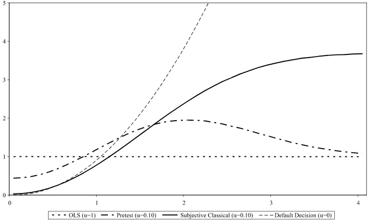
In Figure1we report the risks associated to the pretest and sub-jective classical estimators, withθ˜=0 andα=1,0.10,and 0. We notice that for values ofθ0sufficiently close toθ˜, both OLS
and pretest estimators have higher risk than the subjective clas-sical estimator withα=0.10. This holds also for values ofθ0
around 1, the value at which the risks of the OLS estimator and the default decision coincide. Furthermore, the new estimator has bounded risk (unlessα=0, which corresponds to the de-fault decision) and has always lower risk than the dede-fault deci-sion, except for values ofθ˜ very close toθ0. (In the example shown in Figure1the upper bound for the subjective classical estimator is approximately 3.7.) This is a very appealing fea-ture of our estimator, as it guarantees that it will outperform any given default decision in a precise statistical sense.
The decision maker can control via the confidence levelαthe degree of underperformance whenθ˜is close toθ0. The effect of choosing different values forαis to move the risk function of the subjective classical estimator towards its extremes. The higher the confidence in the default decision (i.e., the lower the
α), the steeper its risk function, converging to the risk of the default decision asα→0. The lower the confidence (i.e., the higher theα), the flatter its risk function, converging to the risk of OLS asα→1.
The lower theα, the better the performance of the new esti-mator for values ofθ0 close toθ˜, and the worse for values of
θ0farther away fromθ˜. This implies that high confidence in the default decisionθ˜pays off if its value is close enough toθ0, but comes at the cost of higher risk wheneverθ˜is far away fromθ0. Notice that in the previous example a default decision based on the OLS estimator would never be rejected by the data (since OLS sets the first derivatives equal to zero), but it would also have no value added. High confidence in a bad default decision, on the other hand, would inevitably result in poor forecasts (in small samples). Therefore, formulating a good default decision may be as important as having a good econometric model.
5. INCORPORATING JUDGMENT INTO CLASSICAL ESTIMATION
In this section we generalize the analysis of the previous sec-tions. We formally define a new estimator which depends on
Figure 1. Risk comparison of different estimators.
a default decision and the confidence associated to it, and es-tablish its relationships with classical estimators. This new esti-mator is obtained by adding a constraint on the first derivatives to the classical optimization problem. We also discuss the rela-tionship with Bayesian econometrics.
As argued in theIntroduction, optimal forecasts maximize the expected utility of the decision maker, which depends on the actions to be taken. Following the framework of Newey and McFadden (1994), denote withUˆT(θ)the finite sample
approx-imation of the expected utility, which depends on the decision variablesθ, data and sample size.θis a vector belonging to the k-dimensional parameter space. We assume the following:
Condition 1(Uniform convergence). UˆT(θ)converges
uni-formly onin probability to U0(θ), that is supθ∈| ˆUT(θ)−
U0(θ)| p
−→0.
Condition 2(Identification). U0(θ)is uniquely maximized
atθ0.
Condition 3(Compactness). is compact. Condition 4(Continuity). U0(θ)is continuous.
These are the standard conditions needed for consistency re-sults of extremum estimators (see theorem 2.1 of Newey and McFadden1994). The classical estimator maximizes the em-pirical expected utility:
Definition 1(Classical estimator). Theclassical estimatoris ˆ
θT=arg maxθUˆT(θ).
Before defining the new estimator, we impose the following conditions:
Condition 5. θ0∈interior().
Condition 6 (Differentiability). UˆT(θ) is continuously
dif-ferentiable.
Convexity of the objective function inθ is needed to ensure consistency, as otherwise the estimator could stop at a local maximum. More precisely convexity is needed because the test for optimality is based on the first order conditions. Since first derivatives describe only local behavior, without the convexity assumption setting the first derivative equal to zero is only a necessary, but not sufficient, condition for optimality. It may be possible to eliminate the convexity assumption by basing the test for optimality on a likelihood ratio test. However, reasoning in terms of first derivatives helps building intuition and motivat-ing the proposed approach. The others are technical conditions typically imposed to derive asymptotic normality results.
Define the following convex linear combination, which shrinks from the default decision θ˜ to the classical estimate ˆ
θT:
θ∗(λ)≡λθˆT+(1−λ)θ˜, λ∈ [0,1]. (6) Denote withˆT a consistent estimate of . Define [note that the test statistic in (7) relies on an asymptotic approximation
to its distribution. If it is suspected that with the available sam-ple size such approximation may be poor, one could resort to bootstrap methods to improve the accuracy of the estimator]:
ˆ
zT(θ∗(λ))≡T∇′θUˆT(θ∗(λ))ˆ−T1∇θUˆT(θ∗(λ)). (7)
Notice that given the realization ofθˆT,θ∗(λ)forλ∈ [0,1] rep-resents a point on the segment joiningθˆT andθ˜. We can, there-fore, test whether any of these points is equal toθ0. Under the null hypothesisH0:θ0=θ∗(λ), we have:
ˆ
zT(θ∗(λ))= ˆzT(θ0) d
−→χk2.
The new estimator is defined as follows:
Definition 2 (Subjective Classical Estimator). Letθ˜ denote the default decision and α∈ [0,1] the confidence level asso-ciated to it. Define θ∗(λ) and zˆT(θ∗(λ)) as in Equations (6)
and (7), respectively, and letηα,k denote theχk2critical value
associated to the confidence level α. The subjective classical estimatorisθ∗(λˆT), where:
This estimator generalizes the estimator found in Equa-tion (5) proposed in Section3 to any objective function sat-isfying Conditions1–8 and to any dimension of the decision variableθ. It first checks whether the given default decisionθ˜ is supported by the data. If for given θ˜ and confidence level
α, the objective function cannot be increased in a statistically significant way, the default decisionθ˜is retained as the forecast estimator. Rejection of the null hypothesis implies that it is pos-sible to move away fromθ˜ and increase (in a statistical sense) the objective function. The classical estimateθˆT (representing the maximum of the empirical equivalent of the objective func-tion) provides the natural direction towards which to move. The new estimator is, therefore, obtained by shrinking the default decision θ˜ towards the classical estimate θˆT. The amount of shrinkage is determined by the constraint in Equation (8) and is given by the point where the increase in the objective function stops being statistically significant. This happens at the bound-ary of the confidence set.
Notice that, as stated at the end of Remark3 in Section3, the constrained maximization problem found in Equation (8) is equivalent to minλ∈[0,1]λ, s.t.zˆT(θ∗(λ))≤ηα,k.
The following theorem shows that the new estimator is con-sistent and establishes its relationship with the classical estima-tor.
Theorem 1(Properties of the subjective classical estimator). Under Conditions1–8the subjective classical estimatorθ∗(λˆT)
of Definition2satisfies the following properties: 1. Ifα=1,θ∗(λˆT)is the classical estimator.
2. Ifα >0,θ∗(λˆT)is consistent.
Proof. SeeAppendix.
The intuition behind this result is that as the sample size grows the distribution of the first derivatives will be more and
more concentrated around its true mean. Since, according to Definition2, the estimator cannot be outside the perimeter of the 1−αconfidence interval, Conditions1–8guarantee that the confidence interval shrinks asymptotically towards zero and, therefore, the consistency of the estimator.
5.1 Relationship With Bayesian Econometrics
An important issue that deserves discussion is the relation-ship between the subjective classical estimator and the Bayesian approach to incorporating judgment. Bayesian estimators re-quire the specification of a prior probability distributionπ(θ). This prior distribution is then updated with the information con-tained in the sample, by applying the Bayes’ rule. The posterior density ofθgiven the sample datayT≡ {yt}Tt=1is given by:
π(θ|yT)=f(y
T|θ)π(θ)
m(yT) ,
wheref(yT|θ)denotes the sampling distribution andm(yT)the
marginal distribution ofyT. In the Bayesian framework, non-sample information is incorporated in the econometric analy-sis via the prior π(θ). Once the prior has been formulated, Bayesian techniques can be applied to find theθˆB
T which
max-imizes the expected utility (see Berger1985and the references cited in Granger and Machina2006for further discussion).
The estimator proposed in this article offers a classical alter-native to Bayesian techniques to account for nonsample infor-mation in forecasting. The nonsample inforinfor-mation is summa-rized by the two parameters(θ˜, α).θ˜ is the agent’s default de-cision, whileαis the confidence level in such a decision, which is then used to test the hypothesisH0:θ˜=θ0, whereθ0
repre-sents the optimal decision variable.
There is one special case in which the two estimators coin-cide. This happens when the decision maker is absolutely cer-tain about the default decisionθ˜. In this case, the prior distrib-ution collapses to a degenerate distribdistrib-ution with total mass on the pointθ˜. With such a prior, the posterior will always be iden-tical to the prior, no matter what the sample data looks like and the Bayesian estimator will be θˆB
T = ˜θ. In our setting, on the
other hand, certainty about parameter values may be expressed by settingα=0. Whenα=0 the null hypothesis can never be rejected and the new estimator becomesθ∗(λˆT)= ˜θ.
A second special case is when the decision maker has no in-formation to exploit, besides that incorporated in the sample. Although this is a highly controversial issue in Bayesian sta-tistics (see for instance Poirier1995, pp. 321–331, and the ref-erences therein), lack of nonsample information can be accom-modated in the Bayesian framework by choosing a diffuse prior. In some special cases—for example when estimating the mean of a Gaussian distribution with known variance—the Bayesian estimator based on a normal prior with variance tending to in-finity is known to converge to the classical estimator. In our setting, instead, lack of information can be easily incorporated by settingα=1, which, as shown in Theorem1, leads to the classical estimator.
For the intermediate cases, there is no obvious mapping be-tween Bayesian priors and our subjective parameters (θ˜, α). The choice between the two estimators depends on how the nonsample information is formalized. Our estimator is not suited to exploit nonsample information which takes the form
of a prior probability distribution, and in this case one needs to resort to Bayesian estimation procedures. On the other hand, application of Bayes’ rule relies on the availability of a fully specified prior probability distribution and if the nonsample in-formation is expressed in terms of the two parameters(θ˜, α), one needs to use the subjective classical estimator. From this perspective, the choice between Bayesian and classical econo-metrics is not an issue to be settled by econometricians, but rather by the decision maker through the format in which she/he provides the nonsample information.
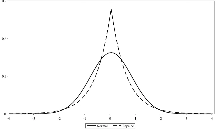
A major potential problem with Bayesian econometrics is that formulation of priors is not always obvious and may, in some cases, put a heavy burden on the decision maker. As an example of such difficulties, consider again the risk analysis of Section4. In Figure2, we compare the risk function of the sub-jective classical estimator with that of two Bayesian estimators, one based on a normal prior and one based on a Laplace (also known as double exponential) prior. We calibrated the priors in such a way that all risk functions intersect at the same point. We see that these two specific Bayesian estimators are dominated by the subjective classical estimator for low and high values of θ0, while the converse is true over a finite intermediate interval. The risk function of the Laplace estimator has an upper bound at around 3.8, while the subjective classical estimator has an upper bound at around 3.7.
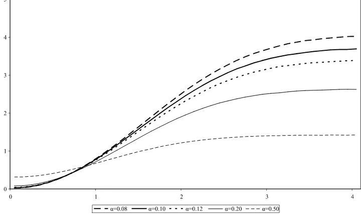
In Figure3, we report the calibrated priors. The Laplace dis-tribution has greater mass around zero and thicker tails with respect to the normal distribution. The tail behavior of the prior distribution leads to estimators with substantially different properties, as shown in Figure2. An undesirable characteristic of the normal Bayesian estimator is that its risk function di-verges to infinity for increasing values ofθ0: there is no limit to the potential damage inflicted by poorly chosen priors. As dis-cussed in Magnus (2002), the unbounded risk is a consequence of the fact that the tails of the normal distribution are too thin. The heavy tails of the Laplace distribution on the other hand guarantee a bounded risk function. The shape of the risk func-tions of the subjective classical estimator on the other hand is not particularly sensitive to small changes ofα, as illustrated in Figure4.
How difficult it is to elicit the tail behavior of the priors de-pends on the knowledge of the decision maker and on the type of problems she/he is facing. These difficulties would be further exacerbated in a multivariate context. The examples discussed in the next section show that the subjective classical estimator instead is relatively straightforward to implement.
6. EXAMPLES
We illustrate with two examples how the theory developed in the previous section can be implemented.
In the first example, we estimate the optimal portfolio weights maximizing a mean-variance utility function. We high-light how the theory proposed in this article naturally takes into account the impact of estimation errors and show, with an out of sample exercise, how the subjective classical estimator out-performs a given benchmark portfolio.
The second example is an application to U.S. GDP forecast. We show how one can map a default decision on future GDP growth rates into default parameters of the econometrician’s fa-vorite model. We provide an illustration using an autoregressive model to forecast quarterly GDP growth rates.
Figure 2. Risk functions of Bayesian estimators with different priors.
6.1 Mean-Variance Asset Allocation
Markowitz’s (1952) mean-variance model provides the stan-dard benchmark for portfolio allocation. It formalizes the in-tuition that investors optimize the trade off between returns and risks, resulting in optimal portfolio allocations which are a function of expected return, variance (the proxy used for risk), and the degree of risk aversion of the decision maker. Despite its theoretical appeal, it is well known that standard implemen-tations of this model produce portfolio allocations with no eco-nomic intuition and little (if not negative) investment value. These problems were initially pointed out, among others, by Jobson and Korkie (1981), who used a Monte Carlo experiment to show that estimated mean-variance frontiers can be quite far away from the true ones. The crux of the problem is
color-fully, but effectively, highlighted by the following quotation of Michaud (1998, p. 3):
“[Mean-variance optimizers] overuse statistically estimated information and magnify the impact of estimation errors. It is not simply a matter of garbage in, garbage out, but, rather, a molehill of garbage in, a mountain of garbage out.”
The problem can be restated in terms of the theory devel-oped in Section 5. Classical estimators maximize the empiri-cal expected utility, without taking into consideration whether they are statistically significantly better than the default de-cision. Our theory provides a natural alternative. For a given benchmark portfolio (the default decisionθ˜ in the notation of Section5) and a confidence levelα, the resulting optimal port-folio is the one which increases the empirical expected utility as long as the first derivatives are statistically different from zero.
Figure 3. Normal and Laplace prior distributions.
Figure 4. Sensitivity of subjective classical estimators to differentαs.
To formalize this discussion, consider a portfolio withN+ 1 assets. Denote withθ theN-vector of weights associated to the first N assets entering a given portfolio, and denote with yt(θ)the portfolio return at time t, where the dependence on
the individual asset weights has been made explicit. Since all the weights must sum to one, note that θN+1=1−Ni=1θi,
whereθi denotes the ith element ofθ andθN+1 is the weight
associated to the (N+1)th asset of the portfolio. Let’s assume an investor wants to maximize a trade-off between mean and variance of portfolio returns, resulting in the following expected utility function:
U(θ)=E[yT+1(θ)] −ξV[yT+1(θ)]
=E[yT+1(θ)] −ξE[y2T+1(θ)] −E[yT+1(θ)]2, (9)
whereξ describes the investor’s attitude towards risk. The em-pirical analogue is:
ˆ
UT(θ)=T−1 T
t=1
yt(θ)
−ξ T−1
T
t=1
y2t(θ)−
T−1
T
t=1
yt(θ) 2
. (10)
The first order conditions are:
∇θUˆ(θ)=T−1
T
t=1
∇θyt(θ)
−ξ T−12
T
t=1
yt(θ)∇θyt(θ)
−2
T−1
T
t=1
yt(θ)
T−1
T
t=1
∇θyt(θ)
,
where∇θyt(θ)≡yNt −y N+1
t ι,yNt is anN-vector containing the
returns at timetof the firstNassets,yNt+1is the return at time
t of the (N +1)th asset, and ι is an N-vector of ones. The variance-covariance matrix of the first derivatives is computed using the outer product estimate.
We apply the methodology developed in Section5to monthly log returns of the stocks composing the Dow Jones Indus-trial Average (DJIA) index, as of July 15, 2005. The sam-ple runs from January 1, 1987 to July 1, 2005, for a total of 225 observations. We set ξ =1 and use as default deci-sion the equally weighted portfolio and confidence levelsα=
1,0.10,0.01. Although any other benchmark could be used, the equally weighted portfolio has emerged as a natural benchmark in the literature. For instance, DeMiguel, Garlappi, and Up-pal (2009) showed that, among 14 estimated models, none of them is consistently better than the naive 1/Nportfolio. Regard-ing the choice of the confidence levelα, recall from Figures1 and4 that it reflects the risk of underperforming with respect to the benchmark portfolio: the lower α, the lower such risk. At the same time the lowerα, the lower the improvement over the benchmark, when the benchmark is far away from the opti-mal portfolio. This dichotomy corresponds to the probability of Type I error (falsely rejecting the null) and Type II error (falsely accepting the null) in hypothesis testing. For a fixed sample, it is not possible to simultaneously reduce both probabilities and the decision maker faces an inevitable trade-off. In the follow-ing example we will useα=0.01 and 0.10, which are values typically used in hypothesis testing.
Notice that the case withα=1 corresponds to the standard implementation of the mean-variance model, i.e., it corresponds to the case where the sample estimates of expected returns and variance-covariances are substituted into the analytical solution of the optimal portfolio weights.
We recursively estimated the optimal weights associated to the different confidence levelsαfor portfolios with a different number of assets, namely, 4, 16,and 30. Following DeMiguel, Garlappi, and Uppal (2009), we evaluate the out of sample per-formance of the estimators using rolling windows ofM=60 andM=120 observations. That is, at each month t, starting
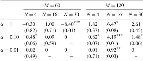
Table 1. Average difference in out of sample realized utilities associated toθ∗(λˆT)and to the equal weighted benchmark. p-values of the Giacomini and White (2006) test of predictive ability in parenthesis. Values significant at the 10%, 5%, and 1%
levels are denoted by one, two, and three asterisks, respectively
M=60 M=120
fromt=M, we estimate the optimal weights using the previ-ousMobservations. Next, we compute the out of sample real-ized return att+1 of the optimal portfolio. With a sample of sizeT, we obtain a total ofT−Mout of sample observations. Finally, we compute average realized utilities associated to the optimal portfolio out of sample returns. In Table1 we report the difference in average utilities between the optimal portfo-lio and the equal weight benchmark. That is, if we denote with Ut(θ)≡yt(θ)−ξ{y2t(θ)− [(T−M)−1
T
t=M+1yt(θ)]yt(θ)}the
realized utility associated to portfolioθ, we compute:
ZT−M≡(T−M)−1
We also compute the test of predictive ability associated to the statisticZT−M, as suggested by Giacomini and White (2006).
We report in parenthesis thep-values associated to the null hy-pothesis that the two portfolios have equal performance.
Let’s look first at the performance of the estimators with a window of 60 observations. We notice that the classical estima-tor (α=1) performs worse than the equal weight benchmark for portfolios with 4 and 30 assets. In the case of the 30 as-set portfolio, the inferior performance of the classical estima-tor is also statistically significant at the 1% confidence level. As we decreaseα, the performance of the estimator improves. With N=4, we see that the optimized portfolio outperforms the benchmark in a statistically significant way forα=0.10. Whenα=0.01, the difference in realized expected utilities is still positive but no longer statistically significant. For the port-folio with 16 assets, none of the optimized portport-folios signifi-cantly outperforms the benchmark. ForN=30, the benchmark is not rejected at the 10% level. (Note that the zeros in the table reflect the fact that the benchmark portfolio is never rejected. In this caseθ∗T= ˜θ and, therefore, the optimized and benchmark portfolios are identical.)
With an estimation window of 120 observations, the perfor-mance of all estimators improves. With a larger estimation sam-ple, estimates become more precise. It is nevertheless interest-ing to notice that the performance of the classical estimator can be improved upon, by reducing the size ofα. WithN=4, the outperformance of the classical estimator is not statistically sig-nificant, while it is withα=0.10. WithN=16, the outperfor-mance of the estimator withα=1 is statistically significant at
the 10% level, but one can increase its significance by reduc-ingαto 0.10. Finally, withN=30, the difference in realized expected utilities is significant only by choosingα=0.10.
What emerges from these results is that the smallerMand the largerN, the greater the impact of estimation error on the op-timal portfolio weights. Consistently with the results discussed in Section4, the lowerα, the more confident the decision maker can be that the resulting allocation will beat the benchmark portfolio. There is, however, no free lunch: choosing too small an α will result in more conservative portfolios (i.e., portfo-lios closer to the benchmark), implying that the decision maker may forgo potential increases in the expected utility. This can be linked back to the discussion of Figure1in Section4. The lowerα, the higher the likelihood that the subjective classical estimator will have lower risk than the default decision (i.e., the risk function of the subjective classical estimator will lie below that of the default decision, except for values ofθ0very close to
˜
θ). At the same time, the lowerα, the higher the risk associated to the subjective classical estimator for values of θ0far away fromθ˜.
6.2 Forecasting U.S. GDP
A possible difficulty in implementing the estimator of Sec-tion5is related to the formulation of a default decision in terms of the parameters of an econometric model about which the de-cision maker may know nothing or very little. We propose a simple strategy to map a default decision on the variable of in-terest to the decision maker (GDP in this case) into default deci-sions on the parameters of the econometrician’s favorite model. In principle, it is possible to express a default decision di-rectly on the parameter vectorθ or indirectly on the dependent variableyT+1to be forecast. If the decision maker can
formu-late a guess onθ, the theory of Section5can be applied directly. In most circumstances, however, it may be more natural to have a judgment about the future behavior ofyT+1, rather than about
abstract model parameters. Let’s denote this default decision as ˜
yT+1. Using the notation of Section5, this can be translated into
default parameters onθas follows: ˜
default parameter vector by choosing theθ˜ that maximizes the objective function subject to the constraint that the forecast at timeTis equal toy˜T+1.
Let’s consider, for concreteness, an application to quarterly GDP forecasting, using an AR(4)model:
yt=θ0+ 4
i=1
θiyt−i+εt. (13)
If the decision maker has a quadratic loss function, we have ˆ
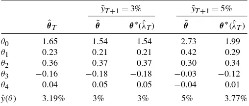
Table 2. Subjective guessesθ˜and estimated parametersθ∗
T(λ)ˆ associated to different subjective guesses on Q4 2005 GDP growth rates (3% and 5%), withα=0.10. A subjective guess of 3% is not rejected by the data and maps into parameter values very close to the
OLSθˆT. A subjective guess of 5%, instead, is rejected by the data, resulting in parameter estimates different from the parameter guess
˜
yt−4]′. We estimate the asymptotic variance-covariance matrix
of the score using standard heteroscedasticity-consistent esti-mators (White1980):
whereθˆT is the OLS estimate. We estimate this model using quarterly data for the U.S. real GDP growth rates. The data are taken from the FREDdatabase (seehttp:// research.stlouisfed. org/ fred2). The data has been seasonally adjusted and our sam-ple runs from Q1 1983 to Q3 2005, with 90 observations. The growth rates are computed as log differences.
For illustratory purposes, we consider two different default decisions for GDP growth in the next quarter (Q4 2005), ˜
yT+1=3% andy˜T+1=5%, both with a confidence levelα=
0.10. The results reported in Table2show thaty˜T+1=3% maps
into a parameter guessθ˜ which cannot be rejected by the data [θ∗(λˆT)= ˜θ]. These parameter values are also very close to the
OLS estimatesθˆT, resulting in very similar forecasts. Note that in this case the forecast associated toθ∗(λˆT)is equal to 3%, the
original default decision (y˜T+1=3%).
The other default decision,y˜T+1=5%, is instead rejected by
the data at the chosen confidence level, resulting in parameter estimatesθ∗(λˆT)which are different from the parameter guess
˜
θ. The estimated shrinkage factorλˆTwas 0.68. The out of
sam-ple GDP forecast at Q4 2005 associated to θ∗(λˆT) is 3.77%
and the OLS forecast is 3.19%, both definitely lower than the default decision of 5%.
7. CONCLUSION
Classical forecasts typically ignore nonsample information and estimation errors due to finite sample approximations. In this article we pointed out how these two problems are con-nected. We explicitly introduced into the classical estimation framework two elements: a default decision and a confidence associated to it. Their role is to explicitly take into considera-tion the nonsample informaconsidera-tion available to the decision maker. These elements served to define a new estimator, which in-creases the objective function only as long as the improvement
is statistically significant, and to formalize the interaction be-tween judgment and data in the forecasting process.
We illustrated with a detailed risk analysis the properties of the new estimator. We provided two applications, which give strong support to our theory. We illustrated how our new es-timator may provide a satisfactory solution to the well-known implementation problems of the mean-variance asset allocation model. We also showed how a default decision on the variable to be forecast can be mapped into default parameters of the econometrician’s favorite model.
APPENDIX
Proof of Theorem1(Properties of the New Estimator)
1. Ifα=1,ηα,k=0 and the constraint in Equation (8)
be-the constraint in Equation (8) and, therefore, a contradic-tion.
ACKNOWLEDGMENTS
I would like to thank, without implicating them, two anony-mous referees, Lorenzo Cappiello, Matteo Ciccarelli, Rob En-gle, Lutz Kilian, Jan Magnus, Benoit Mojon, Cyril Monnet, An-drew Patton and Timo Teräsvirta for their comments and useful suggestions. I also would like to thank the ECB Working Pa-per Series editorial board and seminar participants at the ECB, Tilburg, Federal Reserve Board of Governors, Federal Reserve Bank of Chicago, Oxford, Stanford and UCSD. The views ex-pressed in this paper are those of the author and do not nec-essarily reflect those of the European Central Bank or the Eu-rosystem.
[Received February 2008. Revised May 2009.]
REFERENCES
Berger, J. O. (1985),Statistical Decision Theory and Bayesian Analysis(2nd ed.), New York: Springer-Verlag.
DeMiguel, V., Garlappi, L., and Uppal, R. (2009), “Optimal versus Naive Di-versification: How Inefficient Is the 1/NPortfolio Strategy?”Review of Fi-nancial Studies, 22, 1915–1953.
Durlauf, S. N. (2002), Discussion of “The Role of Models and Probabilities in the Monetary Policy Process,” by C. Sims,Brooking Papers on Economic Activity, 2, 41–50.
Giacomini, R., and White, H. (2006), “Test of Conditional Predictive Ability,” Econometrica, 74, 1545–1578.
Gonzalez, A., Hubrich, K., and Teräsvirta, T. (2009), “Forecasting Inflation With Gradual Regime Shifts and Exogenous Information,” Research Pa-per 2009-3, CREATES.
Granger, C. W. J., and Machina, M. (2006), “Forecasting and Decision Theory,” inHandbook of Economic Forecasting, eds. G. Elliott, C. W. J. Granger, and A. Timmermann, Amsterdam: North-Holland, pp. 81–98.
Granger, C. W. J., and Newbold, P. (1986),Forecasting Economic Time Series, London: Academic Press.
Haavelmo, T. (1944), “Supplement to ‘The Probability Approach in Economet-rics’,”Econometrica Supplemental Material, 12.
Hansen, P. R. (2007), “In-Sample and Out-of-Sample Fit: Their Joint Dis-tribution and Its Implications for Model Selection and Model Averag-ing (Criteria-Based Shrinkage for ForecastAverag-ing),” mimeo, Stanford Univer-sity.
Jobson, J. D., and Korkie, B. (1981), “Estimation for Markowitz Efficient Portfolios,”Journal of the American Statistical Association, 75, 544–554.
Magnus, J. R. (2002), “Estimation of the Mean of a Univariate Normal Distribution With Unknown Variance,” Econometrics Journal, 5, 225– 236.
Magnus, J. R., and Durbin, J. (1999), “Estimation of Regression Coefficients of Interest When Other Regression Coefficients Are of No Interest,” Econometrica, 67, 639–643.
Markowitz, H. M. (1952), “Portfolio Selection,”Journal of Finance, 39, 47–61. Michaud, R. O. (1998), Efficient Asset Allocation. A practical Guide to Stock Portfolio Optimization and Asset Allocation, Boston, MA: Harvard Business School Press.
Newey, W., and McFadden, D. (1994), “Large Sample Estimation and Hypoth-esis Testing,” inHandbook of Econometrics, Vol. IV, eds. R. F. Engle and D. L. McFadden, Amsterdam: Elsevier Science.
Poirier, D. J. (1995),Intermediate Statistics and Econometrics. A Comparative Approach, Cambridge, MA: MIT Press.
White, H. (1980), “A Heteroskedaticity-Consistent Covariance Matrix Esti-mator and a Direct Test for Heteroskedasticity,”Econometrica, 48, 817– 838.