Full Terms & Conditions of access and use can be found at
http://www.tandfonline.com/action/journalInformation?journalCode=ubes20
Download by: [Universitas Maritim Raja Ali Haji] Date: 12 January 2016, At: 23:23
Journal of Business & Economic Statistics
ISSN: 0735-0015 (Print) 1537-2707 (Online) Journal homepage: http://www.tandfonline.com/loi/ubes20
Are Statistical Reporting Agencies Getting It Right?
Data Rationality and Business Cycle Asymmetry
Norman R Swanson & Dick van Dijk
To cite this article: Norman R Swanson & Dick van Dijk (2006) Are Statistical Reporting
Agencies Getting It Right? Data Rationality and Business Cycle Asymmetry, Journal of Business & Economic Statistics, 24:1, 24-42, DOI: 10.1198/073500105000000036
To link to this article: http://dx.doi.org/10.1198/073500105000000036
View supplementary material
Published online: 01 Jan 2012.
Submit your article to this journal
Article views: 88
View related articles
Are Statistical Reporting Agencies Getting It
Right? Data Rationality and Business
Cycle Asymmetry
Norman R. S
WANSONDepartment of Economics, Rutgers University, 75 Hamilton Street, New Brunswick, NJ 08901 (nswanson@econ.rutgers.edu)
Dick
VAND
IJKEconometric Institute, Erasmus University Rotterdam, P.O. Box 1738, NL-3000 DR Rotterdam, The Netherlands (djvandijk@few.eur.nl)
This article provides new evidence on the rationality of early releases of industrial production (IP) and producer price index (PPI) data. Rather than following the usual practice of examining only first available and fully revised data, we examine the entire revision history for each variable. Thus we are able to assess, for example, whether earlier releases of data are in any sense “less” rational than later releases, and when data become rational. Our findings suggest that seasonally unadjusted IP and PPI become rational after approximately 3–4 months, whereas seasonally adjusted versions of these series remain irrational for at least 6–12 months after initial release. For all variables examined, we find evidence that the remaining revision is predictable from its own past or from publicly available information in other economic and financial variables. In addition, we find a clear increase in the volatility of revisions during recessions, suggesting that early data releases are less reliable in tougher economic times. Finally, we explore whether nonlinearities in economic behavior manifest themselves in the form of nonlinearities in the rationality of early releases of economic data, by separately analyzing expansionary and recessionary economic phases and by allowing for structural breaks. These types of nonlinearities are shown to be prevalent and in some cases to lead to incorrect inferences concerning data rationality when they are not taken into account.
KEY WORDS: Efficiency; Nonlinearity; Real-time dataset; Structural change; Unbiasedness.
1. INTRODUCTION
The construction of accurate preliminary announcements of macroeconomic variables remains an area of key interest to pol-icymakers and researchers alike. The reasons for this are many. For example, policymakers have to rely on preliminary esti-mates of key macroeconomic variables when making their de-cisions. Optimal policy depends on accurate assessments of the state of the economy, which implies that the policymakers are interested in whether early releases of data, when viewed as predictions of final or “true” data, may be “rational,” using the terminology of Muth (1961). Similarly, researchers construct-ing empirical models for studyconstruct-ing policy decisions are faced with the task of ensuring that the data used in their analysis cor-respond as closely as possible to those data that policymakers actually had available in real time. This issue is often ignored, because in most cases historical data are used as available at the time when the research is undertaken. Only the most re-cent observations in these data are preliminary releases, corre-sponding with the data available to policymakers. More distant observations, though, are “final” releases, which possibly have undergone substantial revisions over time. Hence the data used ex post by the modeler often are not the same as those used ex ante by the policymaker.
The foregoing notions have led to a huge literature on ex-amining the rationality of late predictions and early releases of macroeconomic variables, as well as the properties of the as-sociated revision processes. A partial list of the many publica-tions in the area include works by Morgenstern (1963), Stekler (1967), Howrey (1978), Zarnowitz (1978), Pierce (1981),
Boschen and Grossman (1982), Mankiw, Runkle, and Shapiro (1984), Mankiw and Shapiro (1986), Mork (1987), Milbourne and Smith (1989), Keane and Runkle (1989, 1990), Diebold and Rudebusch (1991), Neftçi and Theodossiou (1991), Kennedy (1993), Kavajecz and Collins (1995), Mariano and Tanizaki (1995), Rathjens and Robins (1995), Hamilton and Perez-Quiros (1996), Runkle (1998), Gallo and Marcellino (1999), Faust, Rogers, and Wright (2003, in press), Amato and Swanson (2001), Croushore and Stark (2001), Ghysels, Swanson, and Callan (2002), Bernanke and Boivin (2003), and references contained therein. Three main features tie the works in this re-search area together. First, many of them are concerned with either gross domestic product (GDP) or money data. Excep-tions include Diebold and Rudebusch (1991) and Hamilton and Perez-Quiros (1996), who examined the predictive content of the composite leading index for output growth in real time; Keane and Runkle (1990), who evaluated the rationality of price forecasts; and Kennedy (1993), who considered data on the in-dex of industrial production. Second, the focus in many of these articles is on comparing first available (or “preliminary”) data with fully revised (or “final”) data. One reason for this narrow focus is that data on the entire revision process for macroeco-nomic variables have been largely unavailable until recently. From the foregoing list of authors, only Amato and Swanson (2001), Croushore and Stark (2001, 2003), and Bernanke and Boivin (2003) considered complete revision histories for the
© 2006 American Statistical Association Journal of Business & Economic Statistics January 2006, Vol. 24, No. 1 DOI 10.1198/073500105000000036 24
variables that they examined. A further noteable exception to the failure to use revision histories is the seminal article of Keane and Runkle (1990). Keane and Runkle were careful to collect information on what releases of the GDP deflator were available at the dates when forecasts were made, and so revi-sion information was actually in forecasters’ information sets. Third, a common theme in these articles is that the rationality (or lack thereof ) of preliminary data generally is assumed to be constant with respect to the business cycle and constant over time.
In this article we add to the literature on assessing the ra-tionality of preliminary data by examining seasonally adjusted and unadjusted data for industrial production (IP) and the pro-ducer price index for finished goods (PPI). A number of features of our analysis differentiate our work from previous research. First, we have constructed monthly “real-time” datasets that in-clude the entire revision history of the variables that we exam-ine. This means that for each calendar date, we have a complete historical record of the actual values of each variable available at different release dates. Thus we can inspect the entire revi-sion process of the variables in detail, rather than just looking at the properties of first versus final releases of data, for exam-ple. One reason why this is useful is that we are now able to assess whether earlier releases are in any sense “less rational” than later releases. Put another way, we can measure how long it takes before the observed data become rational. In addition, we can include revision histories in the information sets used to examine the rationality of a particular release of data. This al-lows us to assess whether the remaining revision is predictable from its own past, that is, whether revision histories can be used to construct “better” early releases of data.
Second, we recognize that business cycle asymmetry is a stylized characteristic of economic activity, and argue that there is no reason to preclude the possibility that nonlinearities in economic behavior manifest themselves in the form of non-linearities in the revision process or in the rationality of early releases of macroeconomic data (see, e.g., Burns and Mitchell 1946; Shapiro and Watson 1988; Diebold and Rudebusch 1996; King and Watson 1996; Ramsey and Rothman 1996; Baxter and King 1996; Stock and Watson 1999; Granger 2001, and ref-erences therein for discussions of business cycle asymmetry). A number of authors have recognized that nonlinearities may be present in the rationality of preliminary GDP data, including Brodsky and Newbold (1994) and Rathjens and Robins (1995), although they did not examine the entire revision process and did not consider any explicit form of nonlinearity. Our approach is to directly test for the presence of nonlinearities in the re-vision process or in the rationality of early releases based on separate analysis of expansionary and recessionary economic episodes. The distinction between expansionary and recession-ary episodes is useful, because it allows us to determine the extent to which preliminary announcements are accurate in dif-ferent phases of the business cycle. For example, a particular data release may be rational during expansions but irrational during recessions, or vice versa.
Third, there is a growing body of evidence showing that the statistical (business cycle) properties of U.S. macroeco-nomic variables, output and inflation in particular, have changed during the post-World War II period (see, e.g., Watson 1994;
Stock and Watson 1996; McConnell and Perez-Quiros 2000; Blanchard and Simon 2001; Chauvet and Potter 2001; Sensier and van Dijk 2004). The explanations for these changes range from technological change, such as improvements in inventory management and information technology, to improved mone-tary policy. One of our goals in this article is to investigate whether the revision processes of industrial production and in-flation have also been subject to structural breaks. Put differ-ently, we argue that changes in the rationality of early data releases that arise over time may be caused by changes in the data collection and processing techniques used by the statistical agencies. In summary, we wish to shed light on the question of whether government statistics can be made better, and to dis-cuss the “closeness” of preliminary data to final data, an issue of relevance to agents and decision makers who use preliminary data.
We find that seasonally unadjusted IP and PPI releases be-come rational after approximately 3–4 months. Subsequent re-leases do not contain any new information. Seasonally adjusted IP and PPI data, in contrast, remain irrational for at least 6–12 months. For most variables, the past history of the revi-sion process appears useful for ex ante prediction of the remain-ing revision, suggestremain-ing that rules might be constructed for the improvement of early data releases. Furthermore, we find evi-dence of both structural breaks and business cycle asymmetry in the revision process. One noteworthy feature of the revision process is that volatility of early data revisions increases dur-ing recessions, suggestdur-ing that early releases are less reliable in tougher economic times. Not surprisingly, this increase in revision volatility is associated with a general increase in the volatility of the growth rates of our series during recessions, and so is due in part to a general and overall increase in economic uncertainty during contractionary phases of the business cycle. The presence of structural change and nonlinearity in the revi-sion process implies that failure to account for these features may lead to incorrect conclusions concerning data rationality based on linear models. Indeed, we find that rationality of early data releases frequently depends on the stage of the business cycle and has changed over time.
The article is organized as follows. Section 2 contains a sum-mary of the methodology used, as well as a brief discussion of previous research. Section 3 introduces our real-time datasets and discusses the results of an exploratory data analysis describ-ing the main features of the revision processes of our variables. Section 4 contains our main empirical findings, and Section 5 presents conclusions.
2. TESTING DATA RATIONALITY: METHODOLOGY
In what follows we use the following notation. Lett+kXt de-note the value of the (annualized) monthly growth rate of a vari-able of interest that pertains to calendar datetas it is available at timet+k. In this setup, if we assume a 1-month reporting lag, then first release or “preliminary” data are denoted by t+1Xt. In addition, we denote fully revised or “final” data, obtained as k→ ∞, byfXt.
Research in the area of testing rationality of preliminary an-nouncements is based almost exclusively on the framework put forward by Mankiw and Shapiro (1986), linking the first and
final releases of data. Their setup aims to determine whether the first release, t+1Xt, is a noisy estimate of the fully revised data, a rational forecast offXt, or neither of the two. Note that in the first case the revision is uncorrelated with the fully re-vised data, whereas in the second case it is uncorrelated with the first release data. Similarly, in the case where the prelimi-nary announcement is equal to the final data plus measurement error, the variance offXt should be smaller than the variance oft+1Xt, whereas the reverse should hold ift+1Xt is a rational forecast offXt.
Assuming that the value ofXmeasured at timet by the re-porting agency is the value ofXreported at timet, the errors-in-variables hypothesis can be tested by means of the regression model,
t+1Xt=α+fXtβ+εt+1, (1) where εt+1 is an error term assumed to be uncorrelated with fXt. In particular, the null hypothesis thatt+1Xt is equal to fXtplus measurement error is given byα=0 andβ=1.
Using Muth’s (1961) notion of rational expectations, the pre-liminary releaset+1Xtis a rational forecast of the final datafXt if and only if
t+1Xt=E[fXt|t+1], (2) wheret+1is the information set available at timet+1. This possibility can be examined by a second regression model that takes the form
fXt=α+t+1Xtβ+W′t+1γ+εt+1, (3) whereWt+1 is anm×1 vector of variables representing the conditioning information set available at time period t +1 and εt+1 is an error term assumed to be uncorrelated with
t+1Xt andWt+1. The null hypothesis of interest in this model is thatα=0, β=1, andγ =0, based on the notion of
test-ing for rationality of t+1Xt for fXt by determining whether the conditioning information in Wt+1, available in real time
to the data issuing agency, could have been used to construct better conditional predictions of final data. Based on an ex-amination of preliminary and final money stock data, Mankiw et al. (1984) failed to reject the null hypothesis of unconditional unbiasedness using model (1) and found evidence against the null thatα=0,β=1, andγ =0using model (3), suggesting
that preliminary money stock announcements are not rational and are an example of the classical errors-in-variables prob-lem. (For further discussion of the foregoing errors-in-variables hypothesis and rationality hypothesis, see Mankiw et al. 1984; Mankiw and Shapiro 1986; Croushore and Stark 2003; Faust et al., in press, where the errors-in-variables and rational fore-cast models are connected with notions of “noise” and “news.”) As explained by Keane and Runkle (1990), the test of ra-tionality of t+1Xt in the context of model (3) can be broken down into two subhypotheses, namely unbiasedness and effi-ciency. The hypothesis of unbiasedness can be tested by im-posing the restriction thatγ=0and testingα=0 andβ=1, whereas efficiency requires that α=0, β =1, and γ =0.
It is thus not surprising that in the recent literature much at-tention has been focused on model (3). For example, Kavajecz and Collins (1995) found that seasonally unadjusted money an-nouncements are rational, whereas adjusted ones are not. For
GDP data, Mankiw and Shapiro (1986) found little evidence against the null hypothesis of rationality, whereas Mork (1987) and Rathjens and Robins (1995) found evidence of irrationality, particularly in the form of prediction bias [i.e.,α=0 in (3)]. Keane and Runkle (1990) examined the rationality of survey price forecasts rather than preliminary (or real-time) data, us-ing the novel approach of constructus-ing panels of real-time sur-vey predictions. This allowed them to avoid aggregation bias, for example, and may be one reason why they found evidence supporting rationality, even though previous studies focusing on price forecasts had found evidence to the contrary.
One feature of all of the empirical studies discussed thus far is that they used monthly and/or quarterly data. It should be stressed that the distinction between data frequencies is not nec-essarily trivial. For example, models of variables (with differ-ing frequencies) that measure similar economic activity (such as GDP and IP, say) may be approximations of very different underlying data-generating processes with quite different revi-sion characteristics. Thus empirical findings such as ours that are based on monthly data may differ from findings based on examination of quarterly data, for example.
Our approach in this article closely follows that of the afore-mentioned authors, because we also focus on models closely related to model (3). One feature of our approach that differ-entiates it from previous research, however, is that we have the entire revision history for each variable at our disposal, so that we can determine the “timing” of data rationality by generaliz-ing (3) as
fXt−t+kXt=α+t+kXtβ+W′t+kγ+εt+k, (4) wherek=1,2, . . . defines the release of data (i.e., fork=1 we are looking at preliminary data, for k=2 the data have been revised once and so on). Note that in (4), the null hy-potheses of interest are now that α=β =0, assuming that γ =0 (unbiasedness) and α=β =γ =0 (efficiency). Also note thatβ in (4) has a different interpretation fromβ in (3), becauset+kXtis subtracted from both sides of (4) (such that the dependent variablefXt−t+kXt represents the revision remain-ing after thekth data release), and, in (3),k=1. Irrationality of preliminary data releases may arise simply because they are constructed using incomplete information sets. For example, re-leases of aggregate industrial production are based on reported firm production levels. If, say, some firms are “late” in report-ing, then predictions of missing production levels may be used when constructing preliminary data releases, and these predic-tions may be inefficient. Over time, however, as the missing production data become available, newer releases may be ex-pected to be “more” efficient. In this scenario, it follows that after some reasonable amount of time, all subsequent data re-leases are rational. Knowledge of the point in time after which releases of data are efficient has implications for policymak-ers, for example, particularly if they are interested in equating early data releases with efficient predictions of final data. Fi-nally, note that in (4) fork>1, we may defineWt+kto include
characteristics of the revision history, such as the revision be-tween the first andkth releasest+kXt−t+1Xt. In this way, we are able to examine whether inefficiency arises via information available in the revision history for a given release of data, as well as through other sources. Note that a generalization of (4)
is given byt+lXt−t+kXt=α+t+kXtβ+W′t+kγ+εt+k, where k<l. By fitting models of this form, we may examine the ra-tionality of a particular release of data relative to later releases of data. In the following, however, we focus on the model given in (4).
Obviously, inference based on fitting linear regression mod-els of the form given by (4) may be affected by the presence of some form of nonlinearity. In the context of macroeconomic variables, two important types of nonlinearity that also may in-fluence the revision process and rationality of early releases are business cycle asymmetry and structural change. In the remain-der of this section, we describe how we have investigated the relevance of these nonlinearities.
2.1 Data Rationality and the Business Cycle
Our real-time datasets are useful for examining a number of business cycle features of macroeconomic data for which little is known, including asymmetry in the properties of the revi-sion process, in data release rationality, and in the time needed before early releases to become efficient. Asymmetry in the re-vision process or in data release rationality may arise if, for ex-ample, the population of firms changes over the business cycle due to the creation and destruction of firms during expansions and recessions. If early releases of aggregate production levels are based on the same sample of firms irrespective of the stage of the business cycle, then this sample does not accurately rep-resent the underlying population of firms, because young and newly created firms are likely to be underrepresented during ex-pansions and overrepresented during recessions. This may lead to biased early estimates of aggregate production levels in both recessions and expansions, where the sign and magnitude of the bias can be different, implying asymmetry in the revision process and/or rationality of preliminary releases.
As an aside, business cycle asymmetry in data release ef-ficiency may also arise if government reporting agencies are conservative during expansionary periods (e.g., tending to un-derreport economic growth estimates so as not to “overheat” expectations and hence growth), and are liberal during contrac-tionary periods, thereby leading to self-fulfilling cycles of eco-nomic decline (see, e.g., Chauvet and Guo 2003). This would lead to differing levels of efficiency for different observations in the same release of data, depending on whether they pertain to calendar months during expansionary or contractionary peri-ods. The validity of this argument may be questioned given the independence of most statistical offices, however.
Our approach to this issue is to test for asymmetric unbiased-ness and efficiency by fitting models of the form
fXt−t+kXt
=(α1+t+kXtβ1+W′t+kγ1)I[st=0]
+(α2+t+kXtβ2+W′t+kγ2)I[st=1] +εt+k, (5) wherest =0 (or 1) if calendar month t is part of an expan-sion (recesexpan-sion), which is defined using the National Bureau of Economic Research (NBER)-dated business cycle peaks and troughs, and where I[·] is an indicator variable, taking the value 1 if its argument is true and 0 otherwise. But results based on this approach should be viewed only as a rough initial guide
to assessing the importance of asymmetry in our data, because the recession indicator variable is not in agents’ information sets until (usually) after, or close to, the end of the recession. Tests for this type of nonlinearity are all based on checking the equality of coefficients in the foregoing regression model. For example, consider the case where we are only interested in testing unbiasedness in expansions and recessions, so that γ1=γ2=0 is assumed to hold. On rejecting the hypothesis
of linear unbiasedness [α=β=0 in (4) withγ=0imposed],
we test for asymmetry in the (un)biasedness properties by test-ing the null hypothesis α1=α2 andβ1=β2 in (5). In cases where we find such asymmetry, we rerun all of our rationality tests by splitting the data into recessionary and expansionary phases. This allows us to ascertain whether absence of rational-ity in the entire sample is due primarily to a lack thereof during recessionary periods, for example.
2.2 Data Rationality and Structural Change
Structural changes in the revision process or data rationality may be caused by, for example, improvements in data collection and processing methods used by statistical reporting agencies during our sample period (see, e.g., Rathjens and Robins 1995 for further discussion). To explore this possibility, we check for structural changes in the unbiasedness and efficiency test re-gressions. In particular, we use the sup-Wald test as developed by Andrews (1993),
SupW= sup
τ1≤τ≤τ2
WT(τ ), (6)
whereWT(τ )denotes a Wald statistic of the hypothesis of con-stancy of the parameters α and β (and γ) in (4) against the alternative of a one-time change at a fixed break dateτ, given by
fXt−t+kXt
=(α1+t+kXtβ1+W′t+kγ1)I[t< τ]
+(α2+t+kXtβ2+W′t+kγ2)I[t≥τ] +εt+k. (7) The structural change tests are computed by imposing 15% symmetric trimming; that is, we setτ1= [πT]andτ2= [(1−
π )T] +1, with π =.15, where [·] denotes integer part and T is the sample size. The value of τ that minimizes the sum of squared residuals corresponding to (7) is taken to be the es-timate of the break date, denoted byτB. We use the method of Hansen (1997) to obtain approximate asymptoticp values for the sup-Wald test. Note that in principle we should construct p values for our unbiasedness and efficiency regressions using the methodology of Hansen (2000), given that we find evidence for structural change in the revision process. But in our case the distortions to relevantpvalues are small, and so we report only the standardpvalues. Given appropriate estimates of possible break dates, we also construct unbiasedness and efficiency tests on prebreak and postbreak samples, to assess whether our find-ings are driven by nonrobustness of standard efficiency tests to structural change.
Estimation of all models is carried out by least squares, with reported test statistics all based on heteroscedasticity and auto-correlation consistent standard error estimators.
3. REAL–TIME DATA: OVERVIEW AND STATISTICAL PROPERTIES
We have collected seasonally adjusted (SA) and unadjusted (NSA) real-time monthly data for U.S. IP and the PPI for fin-ished goods. The real-time industrial production datasets have been compiled from historical issues of the Federal Reserve Bulletinand theSurvey of Current Business. Recent IP releases also are available at the Federal Reserve Board’s website at http://www.federalreserve.gov/releases/G17/. In addition, a file containing the first five releases of SA IP from 1972:1 on-ward is available on the same site, and the Federal Reserve Bank of Philadelphia recently made available a complete real-time dataset on SA IP athttp://www.phil.frb.org/econ/forecast/ reaindex.html. All of the data for PPI have been gathered from issues of the Survey of Current Business,National Economic Trends, and Business Statistics. Recent data are available at the website of the Bureau of Labor Statistics athttp://stats.bls. gov/ppihome.html.
The number of release dates, or “vintages,” for which we have historical real-time data available varies by series. In par-ticular, for NSA IP, SA IP, and NSA PPI, the first vintage is 1963:1 and the last vintage is 2004:1, with historical data for each vintage going back to 1962:12. For SA PPI, the corre-sponding dates are 1978:2–2004:1 and 1978:1. To facilitate comparison of the results of NSA and SA PPI, we use the NSA data from the vintage of 1978:2 and calendar date 1978:1 onward only. We examine data for calendar periods up until 2001:12, whereas we use the vintage of 2004:1 as our “fully revised” data. Even though we can never claim to have a final record of historical data that is immune from potential future revision, we feel that the difference of 2 years between the last calendar date in our sample period and the date of this vintage is sufficient to consider all observations in this vintage as “fully revised.” This is particularly true because we remove the effect of all benchmark revisions from our data before carrying out unbiasedness and efficiency tests, as we discuss later in this article. Note that although benchmark revisions may include more than just “base year” and “weighting” changes, they are not generally forecastable, justifying their removal in our test regressions reported later.
A typical release of IP data consists of a first release for the previous month and revisions for the preceding 1–5 months (due to the availability of new source data and the revision of source data). In addition, from time to time more compre-hensive rebenchmarking revisions and base-year changes occur that affect the entire (or at least a large part of the) historical time series. During our sample period, base-year changes oc-curred in September 1971, July 1985, April 1990, and Feb-ruary 1997. Further, major revisions due to rebenchmarking occurred in July 1976, May 1993, December 1994, February 1997 (only for the SA series), and annually as of Decem-ber 1997. (See Kennedy 1993; RoDecem-bertson and Tallman 1998; Swanson, Ghysels, and Callan 1999 for additional discussion of the revision process of industrial production.)
The real-time datasets for the PPI involve more infrequent re-vision. In fact, most observations on NSA PPI are revised only once, 3 months after their initial release. The same applies to SA PPI, although for these data additional “periodic” revisions
occur at approximately 12-month intervals (usually in February of each year). These periodic revisions involve incorporating “more comprehensive” information and usually affect data for the preceding 12–15 months. Nonbenchmark revisions do not occur anymore after the first 7 releases for the NSA PPI data and the first 19 releases for the SA PPI data. Finally, there has been no benchmark revision for NSA PPI since 1988, and the base-year was changed only in February 1971 (from 1957–1959 to 1967) and February 1988 (to 1982).
As an aside, it should be stressed that SA data are constructed using seasonal factors that are generally changed only once each year. This feature of the data construction process may account in part for some of the inefficiency in SA data that we discuss subsequently.
Although all data are available in levels, we examine only (annualized) monthly growth rates in this article. This allows us to ignore issues relating to unit roots and cointegration, and also to avoid the problem of accounting for pure base-year changes when comparing multiple revisions of data for a par-ticular calendar date. By a “pure base-year change,” we mean that data are revised only because of a base-year change, with-out regular or definitional revisions occurring at the same time. In addition, the use of growth rates allows for comparison of our findings with those of previous studies. The revision series examined were all tested for a unit root using the augmented Dickey–Fuller test, and all series were found to be covariance-stationary.
As an aside, it is important to note that monthly data of-ten contain more noise than their quarterly counterpart (e.g., IP vs. GDP). Our results reflect this, as can be seen by com-paring the results of various previous quarterly studies, includ-ing those of Keane and Runkle (1990), Croushore and Stark (2001, 2003), Chauvet and Potter (2001), Chauvet and Guo (2003), Chauvet and Popli (in press), and Faust et al. (in press), for example. In addition, it is important to stress that earlier works, such as those of Kennedy (1993), already uncovered ev-idence of inefficiency in the data production process.
We use the following procedure to back out benchmark re-visions from the data. The rere-visions occurring in vintages that are known to involve a comprehensive benchmark revision or base-year change are attributed completely to “benchmark re-visions,” and regular revisions in those vintages are set equal to 0. Of note is that we also used the approach of Kean and Runkle (1990), where benchmark revision was accommodated by using as “final data” those vintages available immediately before benchmark revisions. Interestingly, our findings remain completely unchanged when this approach is adopted, suggest-ing that the two approaches are in some sense interchangeable. Furthermore, when benchmark revision is ignored, test rejec-tions increase markedly, as do regressionR2values, in accord with the findings of Keane and Runkle (1990) demonstrating that failure to account for benchmark revisions can strongly af-fect results. Finally, it should be noted that other benchmark dates were also used to assess the robustness of our findings. These include the set of dates provided by a referee, as well as dates provided in the documentation accompanying the Fed-eral Reserve Bank of Philadelphia real-time IP data. Our results were found to be surprisingly robust to the use of these alterna-tive dating strategies, although the use of fewer dates generally resulted in findings of more inefficiency.
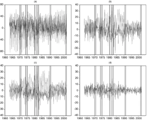
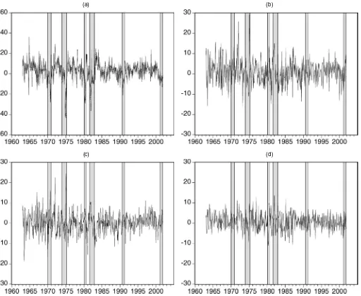
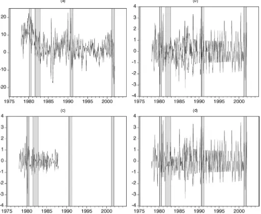
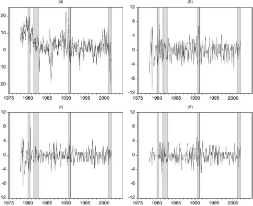
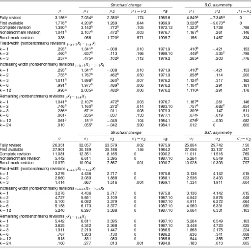
A rough impression of the magnitude of the revisions in IP and PPI can be obtained from the plots given in Figures 1–4. In each figure the first plot is of first available and final release data; the second plot shows the complete revision from the pliminary to the final release; the third plot is of benchmark re-vision, and the last plot is of nonbenchmark revision. Although benchmark revisions often dominate nonbenchmark revisions, both types of revision are rather large relative to the actual val-ues of the series shown in the first plot. The statistical properties of the revision process are analyzed in more detail later.
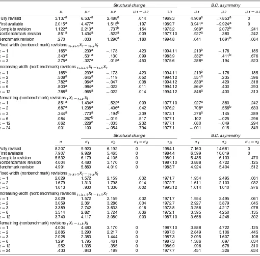
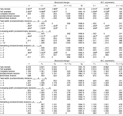
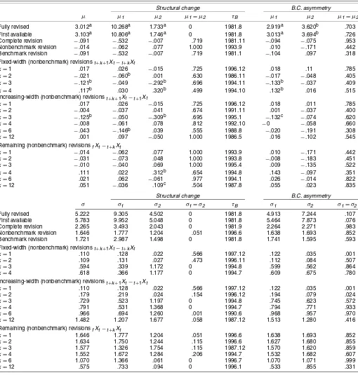
Tables 1–4 report a variety of summary statistics for each variable. These summary statistics include full-sample means of different transformations of the real-time data (see the columns headed “µ”) and means of subsamples determined by application of structural change tests similar to the one dis-cussed in Section 2.2 (see columns headed “µ1 and µ2” un-der “Structural change”), and partitioning the data into those pertaining to calendar months in expansionary phases and re-cessionary phases of the business cycle as defined by NBER turning points (see the columns headed “B.C. asymmetry”).
The lower panel of each table contains similar results for volatilities (denoted by σ,σ1, andσ2). Statistics are reported for fully revised data (fXt), first available data (t+1Xt), com-plete revision (fXt −t+1Xt), and components of the com-plete revision due to “benchmark revisions” (base-year changes and other major revisions) and nonbenchmark or regular sions. In addition, statistics are reported for “fixed-width revi-sions” (i.e.,t+k+1Xt−t+kXt); “increasing-width revisions” (i.e., t+k+1Xt−t+1Xt), and “remaining revisions” (i.e.,fXt−t+kXt). These last three types of data transformations are computed for regular revisions, defined as the remaining revisions after re-moving benchmark revisions from the data, as detailed earlier. Note that “regular revisions” are of particular interest, because these are used in our unbiasedness and efficiency regressions, as discussed later. A number of observations can be made based on these tables.
First, the fully revised (NSA and SA) IP growth rate is con-siderably higher than the preliminary announcement growth rate, on average, whereas for PPI they are very close. Hence re-porting agencies appear to be conservative when rere-porting the
(a) (b)
(c) (d)
Figure 1. Real-Time Monthly Growth Rates of NSA IP. (a) First available (- - - - -) and fully revised (—–) growth rates. (b) Complete revision. (c) Benchmark revision. (d) Nonbenchmark revision.
(a) (b)
(c) (d)
Figure 2. Real-Time Monthly Growth Rates of SA IP. (a) First available (- - - - -) and fully revised (—–) growth rates. (b) Complete revision. (c) Benchmark revision. (d) Nonbenchmark revision.
first release of IP. Note that for IP, the mean nonbenchmark vision is about three times as large as the mean benchmark re-vision, and the latter is not significantly different from 0.
Second, the mean fixed-width, increasing width, and remain-ing revisions for industrial production are often significantly different from 0 (as denoted by superscripts “a,” “b,” and “c,” referring to rejections of the null hypothesis that the mean revi-sion is 0 at the 1%, 5%, and 10% significance levels). As might be expected, there are fewer significant entries in the PPI tables. For example, for the NSA PPI, only the third and fourth fixed-width revision means are significantly different from 0, which is due to the fact that most observations are revised only once, 3 months after initial publication.
Third, both first available and fully revised PPI data are characterized by a structural break in mean, occurring in 1981 (see the first two rows of Tables 3 and 4). For both NSA and SA data, the postbreak mean inflation rate is substantially lower than that for the prebreak period. For IP, evidence in favor of structural breaks in the mean is much weaker, with only the mean of SA fully revised IP data appearing to have possibly
changed, around 1970 (thepvalue of the break test is .174). In-terestingly, though, nonbenchmarkrevisionsfor both NSA and SA IP data do exhibit evidence of a structural break (see the sup-Wald test rejection probabilities in the fourth column of en-tries in Tables 1 and 2). In particular, the mean nonbenchmark revision is considerably smaller in the latter part of the sample (post-1976 for NSA data and post-1977 for SA data), suggest-ing that data collection and processsuggest-ing methods have become more efficient over time.
Fourth, with regard to business cycle asymmetry, notice that inflation is higher and industrial production growth is negative and larger in absolute magnitude during recessionary periods than during expansionary periods (see the last three columns of the tables). Thus the stylized fact that recessions are shorter in duration but greater in intensity is borne out in our datasets. For both NSA and SA IP, the hypothesis of equality of the mean of the complete nonbenchmark revision during expansions and recessions is very close to being rejected. The nonbenchmark revision for calendar months in expansionary periods is about five (three) times larger than for calendar months in
(a) (b)
(c) (d)
Figure 3. Real-Time Monthly Growth Rates of NSA PPI for Finished Goods. (a) First available (- - - - -) and fully revised (—–) growth rates. (b) Complete revision. (c) Benchmark revision. (d) Nonbenchmark revision.
ary periods for NSA (SA) data, whereas the mean nonbench-mark revision for recessionary periods is not significant. Hence it appears that preliminary IP data are correct on average during recessions, but not during expansions. Furthermore, the Fed-eral Reserve is slow in adjusting the growth rate for expan-sionary periods, because the remaining nonbenchmark revision is still significant after the 12th release of data. Finally, note that during recessions, the IP growth rate is adjusted down-ward initially, because on average the first fixed-width revision is negative. This implies that the second release of IP actually is further away from the final data than the first release. This is not the case during expansions.
Fifth, there is rather overwhelming evidence of structural breaks in the volatility of both first available and fully revised data, as well as in revisions. In particular, for IP data, the volatility of both benchmark and nonbenchmark revisions has declined substantially over time, suggesting that preliminary announcements have become more precise and providing fur-ther evidence that data collection and reporting methods have
improved. Note, however, that volatility of nonbenchmark re-visions in NSA PPI data has increased (slightly), suggesting the opposite. The structural change in volatility of first re-lease and fully revised SA IP data occurred in 1984, in agree-ment with McConnell and Perez-Quiros (2000) and others, who reported that the volatility of quarterly GDP has declined since around that time. Similarly, it is not unexpected that the change in volatility of PPI occurred in 1981, after the period of high inflation rates due to the OPEC oil crises in the 1970s.
Sixth, there is evidence that in the IP series there are busi-ness cycle asymmetries in the volatility, not only for first available and fully revised data, but also for revisions. For example, the differential between volatilities in the complete nonbenchmark revision of both NSA and SA IP data dur-ing expansionary and recessionary phases is approximately 25%, with greater volatility occurring during recessions. This finding suggests that uncertainty is different during different phases of the business cycle, and that this difference in
(a) (b)
(c) (d)
Figure 4. Real-Time Monthly Growth Rates of SA PPI for Finished Goods. (a) First available (- - - - -) and fully revised (—–) growth rates. (b) Complete revision. (c) Benchmark revision. (d) Nonbenchmark revision.
certainty has an effect on the reliability of preliminary and early releases of IP data. Put another way, whereas the first release of data may appear to be more accurate on average during recessions, the volatility of revisions demonstrates the opposite pattern. (Recall that the complete nonbenchmark re-vision in IP is substantially larger for calendar months in expansionary periods than for calendar months in recession-ary periods.) Not surprisingly, this increase in revision volatil-ity is associated with a general increase in the volatilvolatil-ity of the growth rates of our series during recessions, and so is due in part to a general and overall increase in economic uncer-tainty during contractionary phases of the business cycle. It is also worth noting that nonbenchmark revision volatility in IP is larger during recessions until the second or third data re-lease. For later releases, this situation is reversed, and there is more uncertainty regarding the remaining revision during expansions.
Finally, after inspecting the correlations between fully re-vised and first available data, we find that NSA first available data are much more highly correlated with their fully revised
counterparts than are the corresponding SA data. For IP, the correlations between first available and fully revised data are approximately .90 for NSA data and .75 for SA data. For PPI, the corresponding correlations are approximately .95 and .90. Thus the seasonal adjustment process itself, which is highly nonlinear (see, e.g., Ghysels, Granger, and Siklos 1996 for dis-cussion of nonlinear aspects of seasonal adjustment filters cur-rently used by statistical reporting agencies) seems to weaken the linkage between first available and final data. Furthermore, regardless of whether or not the data have been seasonally ad-justed, the correlations of both first available and fully revised data with the revisions themselves are often far from 0 and are both positive and negative (correlations in excess of 25% are not uncommon, for example).
Overall, the main conclusion from this exploratory data analysis that carries through to the rest of our analysis is that there is ample evidence of both structural changes and business cycle asymmetries in the revisions to IP and PPI data. This sug-gests that these features may need to be accounted for when testing for unbiasedness and efficiency.
Table 1. Structural Change and Business Cycle Asymmetry in Mean and Volatility: Real-Time Seasonally Unadjusted Industrial Production
Structural change B.C. asymmetry
µ µ1 µ2 µ1=µ2 τB µ1 µ2 µ1=µ2
Fully revised 3.156a 7.034a 2.380a .174 1969.6 4.849a −7.345a 0 First available 1.776b 4.200a 1.269 .644 1969.9 3.526a −9.073a 0 Complete revision 1.380a 3.142a .772a .105 1972.12 1.323a 1.728 .788 Nonbenchmark revision 1.041a 2.107a .472b .003 1976.7 1.167a .261 .146 Benchmark revision .338 .066 1.720b .571 1995.7 .156 1.467 .334 Fixed-width (nonbenchmark) revisionst+k+1Xt−t+kXt
k=1 .295c 1.341a −.008 .010 1971.9 .410b −.421 .153
k=2 .460a .637a .113 .166 1988.10 .448a .535c .798
k=3 .257a .475a .102b .112 1979.2 .265a .203 .776 Increasing-width (nonbenchmark) revisionst+k+1Xt−t+1Xt
k=1 .295c 1.341a −.008 .010 1971.9 .410b −.421 .153
k=2 .755a 1.767a .462b .050 1971.9 .858a .114 .200
k=3 1.011a 1.898a .560b .007 1976.2 1.124a .317 .182
k=6 .991a 1.977a .489b .006 1976.2 1.104a .291 .181
k=12 .996a 2.005a .482b .006 1976.2 1.110a .291 .178 Remaining (nonbenchmark) revisionsfXt−t+kXt
k=1 1.041a 2.107a .472b .003 1976.7 1.167a .261 .146
k=2 .746a 1.160a .272c .014 1983.10 .757a .682c .854
k=3 .286a .671a .011 .008 1979.3 .309a .147 .511
k=6 .061c .235a −.037 .133 1977.1 .074c −.019 .173
k=12 .061c .151a −.045 .104 1984.1 .076b −.030 .082
k=24 .010 .055c −.042 .590 1984.1 .012 0 .600
Structural change B.C. asymmetry
σ σ1 σ2 σ1=σ2 τB σ1 σ2 σ1=σ2
Fully revised 26.351 32.057 23.579 .002 1975.9 25.804 29.742 .150 First available 27.901 30.189 25.186 .146 1984.2 27.056 33.137 .047 Complete revision 11.081 12.351 8.165 0 1990.2 11.011 11.516 .769 Nonbenchmark revision 5.442 6.611 3.395 0 1987.10 5.264 6.549 .103 Benchmark revision 10.079 10.994 7.867 .001 1990.7 10.028 10.393 .797 Fixed-width (nonbenchmark) revisionst+k+1Xt−t+kXt
k=1 3.276 4.436 2.717 0 1975.8 3.136 4.142 .015
k=2 2.660 3.089 1.888 0 1988.1 2.536 3.433 .023
k=3 1.414 .867 1.516 .004 1969.1 1.334 1.911 .004 Increasing-width (nonbenchmark) revisionst+k+1Xt−t+1Xt
k=1 3.276 4.436 2.717 0 1975.8 3.136 4.142 .015
k=2 4.727 5.651 3.109 0 1987.10 4.542 5.876 .048
k=3 5.100 6.082 3.379 0 1987.10 4.911 6.272 .064
k=6 5.158 6.173 3.377 0 1987.10 4.969 6.331 .080
k=12 5.240 6.297 3.388 0 1987.10 5.064 6.331 .103 Remaining (nonbenchmark) revisionsfXt−t+kXt
k=1 5.442 6.611 3.395 0 1987.10 5.264 6.549 .103
k=2 3.625 4.342 2.368 0 1987.10 3.448 4.723 .025
k=3 1.911 2.219 1.447 0 1986.5 1.868 2.175 .224
k=6 .767 1.203 .130 0 1986.2 .836 .341 .008
k=12 .518 .831 .083 0 1985.8 .544 .355 .287
k=24 .160 .277 .013 .001 1984.8 .183 .013 .005 NOTE: The table contains summary statistics for the mean and variance of real-time data on annualized monthly growth rates of NSA IP over the period 1963.1–2001.12, based on data vintages for 1963.1–2004.1. In the upper block, the column headedµcontains the unconditional mean, the columns headedµ1andµ2under “Structural change” contain the means before and after the
breakpointτB, which is determined by maximizing the pointwise heteroscedasticity- and autocorrelation-consistent Wald test for testing the null hypothesisµ1=µ2. Thepvalue corresponding to
the null hypothesis that there was no structural break in the mean of the process is reported in the column headedµ1=µ2. The columns headedµ1andµ2under “B.C. asymmetry” contain the
means during expansions and recessions, which are defined according to NBER business cycle turning points. The column headedµ1=µ2contains thepvalue for the Wald test of equality of
these two means. Entries marked with “a,” “b,” and “c” are significantly different from 0 at the 1%, 5%, and 10% levels, using HAC standard errors. The lower block of the table contains similar statistics for the standard deviations of the time series (computed under the assumption of a constant mean).
4. TESTING DATA RATIONALITY:
EMPIRICAL FINDINGS
In this section we discuss results based on regression mod-els of the form given in (4), (5), and (7). In these regression models,Wt+kincludes the revision between the first andkth
re-lease of data (t+kXt−t+1Xt), the 3-month Treasury bill (T-bill) rate, the spread between yields on 10-year Treasury bonds and 3-month T-bills, the spread between Baa and Aaa rated
cor-porate bonds, the monthly change in logged crude oil prices (West Texas Intermediate Crude), and the monthly dividend reinvested return on the S&P500. These variables are similar to those used by previous authors (noted earlier), who have pro-vided more detailed motivation for their use. All conditioning variables (except of courset+kXt−t+1Xt) are measured at the end of montht+k−1. In addition, and because IP revisions generally occur for the previous three observations, we include fixed-width revisions for these most recent observations
Table 2. Structural Change and Business Cycle Asymmetry in Mean and Volatility: Real-Time SA IP
Structural change B.C. asymmetry
µ µ1 µ2 µ1=µ2 τB µ1 µ2 µ1=µ2
Fully revised 3.137a 6.537a 2.488a .014 1969.3 4.909a −7.853a 0 First available 2.015a 4.477a 1.515b .197 1969.7 3.941a −9.924a 0 Complete revision 1.122a 2.213a .737b .154 1973.2 .969a 2.072b .241 Nonbenchmark revision .851a 1.434a .522a .009 1977.10 .927a .380 .242 Benchmark revision .270 .033 1.296a .180 1994.8 .041 1.691b .064 Fixed-width (nonbenchmark) revisionst+k+1Xt−t+kXt
k=1 .165c .239a −.173 .423 1994.11 .219b −.176 .185
k=2 .343a .531a .130 .099 1983.9 .332a .411b .676
k=3 .275a .327a .015a .450 1975.6 .288a .194 .523 Increasing-width (nonbenchmark) revisionst+k+1Xt−t+1Xt
k=1 .165c .239a −.173 .423 1994.11 .219b −.176 .185
k=2 .508a .645a −.119 .052 1994.12 .551a .235 .396
k=3 .782a .964a −.047 .008 1994.12 .839a .429 .318
k=6 .803a .984a −.022 .011 1994.12 .864a .430 .293
k=12 .788a .965a −.022 .014 1994.12 .846a .430 .313
Remaining (nonbenchmark) revisionsfXt−t+kXt
k=1 .851a 1.434a .522a .009 1977.10 .927a .380 .242
k=2 .687a 1.238a .406a .042 1976.2 .708a .556b .633
k=3 .344a .773a .194b .339 1973.1 .376a .145 .289
k=6 .084 .267b −.019 .517 1977.1 .102 −.025 .296
k=12 .062 .228c −.033 .232 1977.1 .080 −.049 .294
k=24 .001 .100 −.054 .794 1977.1 −.001 .015 .849
Structural change B.C. asymmetry
σ σ1 σ2 σ1=σ2 τB σ1 σ2 σ1=σ2
Fully revised 8.207 9.920 6.192 0 1984.1 7.163 14.681 0 First available 7.907 9.929 5.465 0 1984.4 6.599 16.019 0 Complete revision 5.532 6.179 4.105 0 1989.1 5.435 6.133 .470 Nonbenchmark revision 4.004 4.480 3.170 0 1987.10 3.888 4.722 .125 Benchmark revision 4.991 5.860 4.019 0 1983.7 4.924 5.404 .512 Fixed-width (nonbenchmark) revisionst+k+1Xt−t+kXt
k=1 2.029 1.572 2.159 .032 1971.7 1.954 2.495 .061
k=2 1.679 1.313 1.798 .014 1972.7 1.611 2.103 .032
k=3 1.013 .930 1.336 .002 1993.12 1.014 1.010 .976 Increasing-width (nonbenchmark) revisionst+k+1Xt−t+1Xt
k=1 2.029 1.572 2.159 .032 1971.7 1.954 2.495 .061
k=2 3.059 2.361 3.286 .004 1972.7 2.927 3.879 .045
k=3 3.389 2.742 3.633 .016 1973.8 3.256 4.217 .078
k=6 3.514 2.821 3.724 .036 1972.1 3.395 4.250 .135
k=12 3.740 4.117 3.080 .003 1987.10 3.658 4.248 .302 Remaining (nonbenchmark) revisionsfXt−t+kXt
k=1 4.004 4.480 3.170 0 1987.10 3.888 4.722 .125
k=2 2.885 3.290 2.217 0 1987.3 2.849 3.106 .445
k=3 2.028 2.383 1.444 0 1987.3 2.095 1.607 .108
k=6 1.291 1.795 .461 0 1987.3 1.386 .697 .034
k=12 .952 1.335 .355 0 1986.9 .996 .678 .310
k=24 .433 .843 .189 0 1977.7 .451 .326 .634
NOTE: The table contains summary statistics for the mean and variance of real-time data on annualized monthly growth rates of SA IP over the period 1963.1–2001.12, based on data vintages for 1963.1–2004.1. See Table 1 for further details.
taining to monthst+k−2,t+k−3, andt+k−4 in the set of control variables. As mentioned earlier, for the unbiasedness tests, we always imposeγ =0 orγ1=γ2=0 in the appro-priate regression models. In the efficiency regressions, we also include a set of centered seasonal dummies. In particular, we include11
s=1δsD∗s,t, whereD∗s,t=Ds,t−D12,t, withDs,t=1 if time periodtcorresponds to monthsandDs,t=0 otherwise. Note that the coefficientδsmeasures the difference between the intercept in monthsand the average intercept,α. The seasonal effect for December can be computed asδ12= −11s=1δs, and hence, by construction, it holds that12
s=1δs=0. As a measure of the importance of seasonal effects, we reportδ∗≡12
s=1δˆ2s
in the tables. Including seasonal dummies in the unbiasedness regressions does not yield qualitatively different results from those reported here. Tabulated results are available on request from the authors.
As an aside, we also constructed efficiency tests withWt+k
defined to contain all variables measured at the end of cal-endar month t, regardless of the value of k. These types of tests allowed us to determine the length of time needed be-fore all useful information available at the time of first re-lease is incorporated into the revised data. In addition, we tried settingWt+k=t+kXt−t+1Xt (i.e., including only the re-vision between the first andkth releases of data, to focus on the forecastability of the revision process from its own past).
Table 3. Structural Change and B.C. Asymmetry in Mean and Volatility: Real-Time NSA PPI
Structural change B.C. asymmetry
µ µ1 µ2 µ1=µ2 τB µ1 µ2 µ1=µ2
Fully revised 2.997a 10.046a 1.686a 0 1981.10 2.915a 3.553b .739 First available 2.992a 9.986a 1.691a 0 1981.10 2.906a 3.559b .724 Complete revision .005 −.010 .053 1.000 1996.4 .009 −.026 .799 Nonbenchmark revision 0 −.036 .024 1.000 1987.6 .002 −.010 .922 Benchmark revision .011 .121 −.030 .928 1980.9 .019 −.026 .683 Fixed-width (nonbenchmark) revisionst+k+1Xt−t+kXt
k=1 −.001 −.005 0 .992 1985.6 −.002 0 .311
k=3 −.463a −1.517a −.229b 0 1982.5 −.395a −.907a .073
k=4 .464a 1.533a .233b 0 1982.4 .408a .831a .181 Increasing-width (nonbenchmark) revisionst+k+1Xt−t+1Xt
k=1 −.001 −.005 .992 1985.6 −.002 0 .311
k=3 −.464a −1.517a −.231b 0 1982.5 −.397a −.907a .074
k=4 0 −.016 .053 1.000 1996.4 .012 −.076 .478
k=6 −.011 −.082 .019 .964 1985.1 −.011 −.010 .998
k=12 0 −.036 .024 1.000 1987.6 .002 −.010 .922
Remaining (nonbenchmark) revisionsfXt−t+kXt
k=1 0 −.036 .024 1.000 1987.6 .002 −.010 .922
k=2 .002 −.045 .021 1.000 1985.1 .003 −.010 .912
k=3 .464a 1.522a .236b 0 1982.4 .398a .897a .131
k=4 −0 −.017 .007 1.000 1985.1 −.010 .066 .230
k=6 .011 .073 0 .684 1981.8 .013 0 .150
Structural change B.C. asymmetry
σ σ1 σ2 σ1=σ2 τB σ1 σ2 σ1=σ2
Fully revised 6.205 9.831 5.530 0 1981.10 5.829 8.668 .016 First available 6.239 9.714 5.593 0 1981.10 5.913 8.376 .046 Complete revision 1.189 1.301 1.098 .523 1988.10 1.190 1.183 .971 Nonbenchmark revision 1.116 .927 1.191 .320 1984.11 1.133 1.001 .478 Benchmark revision .688 .933 .522 .001 1982.1 .672 .754 .656 Fixed-width (nonbenchmark) revisionst+k+1Xt−t+kXt
k=1 .004 .007 .002 .724 1985.6 .004 .002 .311
k=3 1.241 1.596 1.178 .079 1981.8 1.224 1.348 .375
k=4 1.246 1.587 1.184 .091 1981.9 1.240 1.284 .802 Increasing-width (nonbenchmark) revisionst+k+1Xt−t+1Xt
k=1 .004 .007 .002 .724 1985.6 .004 .002 .311
k=3 1.239 1.595 1.176 .078 1981.8 1.222 1.348 .369
k=4 1.110 .929 1.184 .346 1985.1 1.123 1.019 .566
k=6 1.130 .973 1.193 .554 1984.11 1.150 1.001 .426
k=12 1.116 .927 1.191 .320 1984.11 1.133 1.001 .478 Remaining (nonbenchmark) revisionsfXt−t+kXt
k=1 1.116 .927 1.191 .320 1984.11 1.133 1.001 .478
k=2 1.118 .927 1.194 .307 1984.11 1.136 1.002 .471
k=3 1.118 .927 1.194 .307 1984.11 1.136 1.002 .471
k=4 1.273 1.754 1.186 .004 1981.9 1.264 1.336 .685
k=6 .056 .303 .013 0 1981.8 .063 .013 .031
NOTE: The table contains summary statistics for the mean and variance of real-time data on annualized monthly growth rates of the NSA PPI for finished goods over the period 1978.2–2001.12, based on data vintages for 1978.2–2004.1. The reason for not includingk=2 andk=12 in some of the tables is that all revisions for these values ofkare identically 0. See Table 1 for further details.
These alternative efficiency tests led to qualitatively similar conclusions to those reported herein. Therefore, detailed re-sults are not given here, but are available on request from the authors.
4.1 Linear Models
The basic test of unbiasedness involves testing the null hy-pothesis thatα=β=0 in (4), while imposing the restriction that γ =0. Probability values for Wald tests of this null are given in the fifth column of entries in Tables 5 and 6 headed “α=0 β=0.” Based on a rejection probability value of .10 (which is used in all subsequent discussions), for NSA IP we see that there is bias in the first through third releases of data
and none thereafter. Thus reporting agencies seem to “get it right” on average after the first three revisions. The bias in SA IP (which is due mainly to the interceptαbeing non-0; cf. Mork 1987; Rathjens and Robbins 1995) persists much longer (i.e., approximately 12 months). One reason for this finding may be the very nature of the seasonal adjustment process. In particular, seasonal adjustment procedures make use of two-sided moving average filters, with one side using historical data and the other side using as-yet-undetermined future data. If the filters place enough weight on data that are not known with certainty for a full year or more, this could account for the increase in bias. In summary, although it is known that preliminary data are often biased, we now have evidence that the bias remains prevalent for multiple months of new releases
Table 4. Structural Change and B.C. Asymmetry in Mean and Volatility: Real-Time SA PPI for Finished Goods
Structural change B.C. asymmetry
µ µ1 µ2 µ1=µ2 τB µ1 µ2 µ1=µ2
Fully revised 3.012a 10.268a 1.733a 0 1981.8 2.919a 3.620b .703 First available 3.103a 10.806a 1.746a 0 1981.8 3.013a 3.694b .726 Complete revision −.091 −.532 −.007 .719 1981.11 −.094 −.075 .953 Nonbenchmark revision −.014 −.062 .077 1.000 1993.9 .010 −.171 .442 Benchmark revision −.091 −.532 −.007 .719 1981.1 −.104 .097 .318 Fixed-width (nonbenchmark) revisionst+k+1Xt−t+kXt
k=1 .017 .026 −.015 .725 1996.12 .018 .11 .785
k=2 −.021 −.060b .001 .630 1986.11 −.017 −.048 .405
k=3 −.121b −.049 −.292b .696 1994.11 −.133b −.037 .409
k=4 .117b .030 .320b .499 1994.10 .132b .016 .515 Increasing-width (nonbenchmark) revisionst+k+1Xt−t+1Xt
k=1 .017 .026 −.015 .725 1996.12 .018 .011 .785
k=2 −.004 −.037 .041 .674 1991.11 .001 −.037 .400
k=3 −.125b −.050 −.309b .695 1995.1 −.132c −.074 .620
k=4 −.008 −.061 .078 .812 1992.10 −0 −.058 .660
k=6 −.043 −.146b .039 .555 1988.8 −.020 −.191 .308
k=12 .001 .097 −.050 1.000 1986.5 .016 −.102 .545
Remaining (nonbenchmark) revisionsfXt−t+kXt
k=1 −.014 −.062 .077 1.000 1993.9 .010 −.171 .442
k=2 −.031 −.073 .048 1.000 1993.8 −.008 −.183 .451
k=3 −.010 −.040 .069 1.000 1995.4 .009 −.135 .522
k=4 .111 .022 .312b .654 1994.8 .143 −.097 .351
k=6 .021 .062 −.061 .977 1994.1 .026 −.014 .822
k=12 .051 −.036 .109c .504 1987.8 .055 .023 .835
Structural change B.C. asymmetry
σ σ1 σ2 σ1=σ2 τB σ1 σ2 σ1=σ2
Fully revised 5.222 9.305 4.502 0 1981.8 4.913 7.244 .107 First available 5.783 9.952 5.048 0 1981.8 5.464 7.873 .076 Complete revision 2.265 3.493 2.043 0 1981.9 2.264 2.271 .983 Nonbenchmark revision 1.646 1.777 1.204 .051 1996.6 1.638 1.693 .852 Benchmark revision 1.721 2.987 1.498 0 1981.8 1.741 1.595 .593 Fixed-width (nonbenchmark) revisionst+k+1Xt−t+kXt
k=1 .110 .128 .022 .566 1997.12 .122 .035 .001
k=2 .109 .131 .027 .473 1996.11 .112 .084 .507
k=3 .594 .339 1.172 0 1994.8 .599 .562 .864
k=4 .618 .366 1.177 0 1994.7 .609 .675 .780
Increasing-width (nonbenchmark) revisionst+k+1Xt−t+1Xt
k=1 .110 .128 .022 .566 1997.12 .122 .035 .001
k=2 .179 .219 .024 .154 1996.12 .194 .079 .024
k=3 .729 .523 1.197 0 1994.8 .745 .623 .572
k=4 .791 .531 1.368 0 1994.7 .794 .771 .933
k=6 .966 .694 1.260 .001 1990.6 .968 .957 .970
k=12 1.482 1.207 1.677 .058 1987.12 1.513 1.280 .416 Remaining (nonbenchmark) revisionsfXt−t+kXt
k=1 1.646 1.777 1.204 .051 1996.6 1.638 1.693 .852
k=2 1.634 1.750 1.244 .115 1996.6 1.627 1.680 .855
k=3 1.577 1.326 1.754 .115 1987.12 1.570 1.620 .859
k=4 1.552 1.672 1.284 .206 1994.7 1.532 1.682 .607
k=6 1.070 1.366 .061 0 1996.7 1.070 1.071 .999
k=12 .575 .733 .094 0 1996.1 .533 .855 .331
NOTE: The table contains summary statistics for the mean and variance of real-time data on annualized monthly growth rates of the SA PPI for finished goods over the period 1978.2–2001.12, based on data vintages for 1978.2–2004.1. See Table 1 for further details.
and for a year or more with SA data. This suggests that if one’s objective is to use timely unbiased data, then NSA data are preferable (see Kavajecz and Collins 1995 for an exten-sive discussion of this topic). Even more interesting, note that NSA PPI is essentially unbiased across all releases, except the fourth release (for the reasons explained earlier—i.e., revision usually occurs only 3 months after initial release). However, SA PPI is biased at all releases up to 12 months. (Note that here the coefficientβ also is significantly different from 0, in contrast with the results for SA IP.) Thus even a full year of
revisions is not sufficient to ensure that SA PPI releases are unbiased.
Of note is that many of the unbiasedness regression mod-els have serially correlated and conditionally heteroscedastic errors, according to Breusch–Godfrey serial correlation and autoregressive conditional heteroscedasticity (ARCH) tests, which are reported in the working paper version of this arti-cle (Swanson and van Dijk 2003). This suggests that regression coefficients may be biased and that the regression models may be misspecified, a problem that persists even when Wt+k is
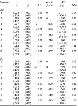
Table 5. Unbiasedness of Real-Time Growth Rates of IP: Linear Model NOTE: The table contains unbiasedness test results for different releases of annualized monthly growth rates of IP over the period 1963.1–2001.12, based on data vintages for 1963.1–2004.1 and based on estimating equation (4) withγ=0 imposed. The column headed “α=0β=0” contains thepvalue of the Wald statistic for testing the indicated restriction. The column headed SC contains thepvalue from the sup-Wald test for testing the hypothesis α1=α2andβ1=β2in (7) withγ1=γ2=0 imposed, where the changepoint,τB, is given in parentheses. The column headed BCA contains thepvalue from the Wald test for testing the hypothesisα1=α2andβ1=β2in (5) withγ1=γ2=0 imposed, using NBER-defined
reces-sions and expanreces-sions. For all test statistics, heteroscedasticity and autocorrelation-consistent versions are used. Additionally, heteroscedasticity and autocorrelation-consistent standard er-rors are given in parentheses under the coefficient estimates.
included in the regression model for the purpose of testing effi-ciency of early releases.
The structural change tests reported in the sixth column of the tables, headed “SC (τB),” suggest that there is a structural break in the revision process for SA PPI in 1981, regardless of data release. In contrast, there is no evidence of structural breaks in the adjusted IP data, and for unadjusted IP and PPI data, all evidence of structural breaks is in the early data releases.
Our tests for business cycle asymmetry reported in the last column of the tables, headed “BCA,” provide moderate evi-dence of such nonlinearity for NSA IP, strong evievi-dence for SA IP, moderate evidence for NSA PPI, and no evidence for SA PPI. Interestingly, there is no evidence of business cycle asymmetry in the NSA PPI regressions whenk=1 (i.e., based on the use of preliminary data in the unbiasedness regressions). Rather, business cycle asymmetry becomes more apparent af-terthe preliminary data have been revised once (which, from our foregoing discussion, we know happens after an interval of approximately 4 months).
Tables 7 and 8 present efficiency test results in the eighth col-umn [tests of the hypothesis thatγ=0 in (4)] and the 10th
col-Table 6. Unbiasedness of Real-Time Growth Rates of the PPI for Finished Goods: Linear Model NOTE: The table contains unbiasedness test results for different releases of annualized monthly growth rates of the PPI for finished goods over the period 1978.2–2001.12, based on data vintages for 1978.2–2004.1. Note thatk=12 is not added to the top panel, because revi-sions are in this case equal to 0 for all observations. For the same reason,k=12 is not added to the results in Table 10. See Table 5 for further details.
umn (tests of the hypothesis thatα=β=γ =δ=0). When testing for seasonality alone (see the 12th column in the lin-ear efficiency tables, headed “δ=0”),revisionsfrom SA data appear to exhibit seasonality. Given that we already have re-sults on the unbiasedness of our data, we now focus on the joint hypothesis of unbiasedness and efficiency (i.e., α=β =γ = δ=0). For this hypothesis, early releases of NSA IP become efficient after 3 months, whereas efficiency is realized for SA IP data after 3–4 months. Recall, though, that when only biased-ness is tested for, the SA data remain biased even after data have been revised 12 times. This is true even though no fur-therirrationality is found to be due to missing information after 3–4 months. The reason for this finding may be thatWt+k
en-ters into the regression models linearly, whereas the seasonal adjustment filter applied to the NSA data is highly nonlinear. In addition, note that the finding that it takes approximately 3 months before NSA IP data are not only unbiased but also efficient suggests that another sort of rationality test could be performed, by checking how many releases of IP data have an impact on returns in the stock market, say. If more than three releases have an impact, then this would suggest that agents are irrational, in the sense that they need not have used additional releases of IP when forming their expectations, because earlier releases were already fully rational. An assessment of rational-ity based on this argument is left for future research.
NSA price data also become efficient after three or four data releases, whereas SA price data are efficient only after 6 months. Unreported alternative efficiency tests that include
38
Jour
nal
of
Business
&
Economic
Statistics
,
J
an
uar
y
2006
Table 7. Efficiency of Real-Time Growth Rates of IP: Linear Model
Tests of efficiency Tests for structural change Tests for B.C. asymmetry
Release k
α=0 α=β=0 α,β α,β
α β γ δ∗ R2 β=0 γ=0 δ=0 γ=δ=0 α,β γ δ γ,δ α,β γ δ γ,δ
NSA
1 2.323 −.032 5.952 .035 .006 .106 .004 0 .052 .021 .369 0 .221 0 0 0
(.788) (.026) (1976.2)
2 .483 −.009 .251 3.374 .061 .488 .001 .003 0 .810 0 .108 0 .432 .025 .004 0
(.494) (.014) (.053) (1976.2)
3 .411 .001 .046 .767 .022 .250 .063 .750 .003 .173 .176 .111 0 .066 0 .017 0
(.261) (.009) (.031) (1982.3)
4 .337 −.007 .050 .726 .016 .098 .048 .703 .360 .250 .004 .268 .020 .011 .039 .884 .403
(.168) (.007) (.019) (1973.4)
5 .135 −.009 .035 .774 .016 .313 .069 .478 .404 .055 .009 .168 .001 .140 .337 .849 .847
(.140) (.007) (.017) (1976.2)
6 .172 −.009 .037 .795 .007 .236 .308 .608 .763 .009 .184 .273 .280 .349 .685 .840 .956
(.139) (.006) (.017) (1976.2)
12 .026 −.004 .028 .668 .025 .554 .212 .180 .246 .181 .313 .188 .277 .938 .268 .527 .418
(.128) (.004) (.011) (1980.4)
24 .013 −.003 .007 .430 .004 .551 .763 .967 .997 .425 .796 .855 1.000 .394 .783 .965 .997
(.031) (.002) (.007) (1984.1)
SA
1 1.406 −.030 3.086 .064 .089 .002 .007 0 0 0 0 0 .499 0 .001 0
(.666) (.029) (1986.1)
2 .848 −.029 .337 2.470 .100 .020 0 0 0 .041 0 0 0 .177 .115 .001 0
(.360) (.016) (.059) (1986.1)
3 .669 −.015 .070 1.217 .015 .041 .021 .085 0 .994 .030 .327 0 0 .331 .001 0
(.288) (.013) (.054) (1973.4)
4 .409 −.021 .027 .978 −.004 .069 .404 .183 .061 .310 0 .082 0 .001 .907 .446 .051
(.240) (.012) (.031) (1973.3)
5 .478 −.024 .024 .830 −.007 .026 .412 .449 .143 .055 .012 .115 0 .023 .968 .480 .417
(.253) (.011) (.028) (1968.10)
6 .338 −.024 .015 .721 −.011 .069 .591 .730 .458 .092 .010 .415 .011 .053 .401 .629 .131
(.234) (.012) (.028) (1968.10)
12 .269 −.018 0 .792 .001 .084 .377 .412 .396 .971 .762 .024 .204 .042 .416 .286 .045
(.209) (.009) (.026) (1984.12)
24 .085 −.008 −.019 .533 −.019 .354 .823 .832 .969 .603 .648 .219 .463 .214 .779 .825 .985
(.196) (.005) (.029) (1968.10)
NOTE: The table contains efficiency test results for different releases of annualized monthly growth rates of IP over the period 1963.1–2001.12, based on data vintages for 1963.1–2004.1 and based on estimating equation (4) withWt+kdefined to include the increasing
width revision up to thekth release of data (i.e.,t+kXt−t+1Xt), the fixed-width revisions for the three most recent observations pertaining to monthst+k−2,t+k−3, andt+k−4, the 3-month T-bill rate, the spread between yields on 10-year Treasury bonds and
3-month T-bills, the spread between Baa and Aaa rated bond yields, the first difference of the logged oil price, and the return on the S&P 500, all observed at the end of montht+k−1. The column with headerγcontains estimates of the coefficient associated with the regressort+kXt−t+1Xt. The column with headerδ∗contains values of
12
s= 1δˆ2s, whereδsˆ is the estimated coefficient forDs,t,s=1, . . . , 11, andδˆ12= −11s= 1δsˆ, which measures the magnitude of seasonal patterns in the revision process. The remainder of the columns contain statistics that correspond to those reported in the previous tables. See Table 5 for further details.