00074918.2013.772941

(1)

Full Terms & Conditions of access and use can be found at

http://www.tandfonline.com/action/journalInformation?journalCode=cbie20

Download by: [Universitas Maritim Raja Ali Haji] Date: 17 January 2016, At: 23:40

ISSN: 0007-4918 (Print) 1472-7234 (Online) Journal homepage: http://www.tandfonline.com/loi/cbie20

Towards a better measure of income inequality in

Indonesia

Kunta Nugraha & Phil Lewis

To cite this article: Kunta Nugraha & Phil Lewis (2013) Towards a better measure of income inequality in Indonesia, Bulletin of Indonesian Economic Studies, 49:1, 103-112, DOI: 10.1080/00074918.2013.772941

To link to this article: http://dx.doi.org/10.1080/00074918.2013.772941

Published online: 21 Mar 2013.

Submit your article to this journal

Article views: 702

View related articles

(2)

Bulletin of Indonesian Economic Studies, Vol. 49, No. 1, 2013: 103–12

*_{The authors are grateful to Tesfaye Gebremedhin, Muni Perumal, Yogi Vidyattama,} Ri-yana Miranti and Ross McLeod for their valuable and helpful comments. We also received many comments from participants at the 40th_{Australian Conference of Economists, in} 2011. Responsibility for the inal version is that of the authors.

TOWARDS A BETTER MEASURE OF

INCOME INEQUALITY IN INDONESIA

Kunta Nugraha* Phil Lewis*

University of Canberra

Indonesia has experienced signiicant economic growth in recent years (on aver -age, 5% in 2000–08), but many people are still living in poverty. Income inequality, as measured by the oficial Gini coeficient, has also increased. This paper evalu -ates household income and income inequality in Indonesia, assessing both market and non-market income to reach a more accurate measure of how actual income affects living standards. We ind that if household income considers non-market in -come, income distribution is signiicantly more balanced, the coeficient of income inequality falls from 0.41 to 0.21 and the income share of the population’s poorest deciles increases more than ivefold. The results suggest that market income alone is a misleading measure of income distribution in Indonesia.

Keywords: net income, actual income, income distribution, income in kind, consumption

of own production

INTRODUCTION

According to Badan Pusat Statistik (BPS), Indonesia’s Central Statistics Agency,

15.4% of Indonesia’s population, or around 35 million people, were poor in 2008,

a percentage that has since decreased (BPS 2010). At the time, BPS set the poverty

line, or the basic-needs approach for food and non-food, at Rp 182,636 per capita per month, or $33.80 using purchasing-power parity (PPP). Indonesia’s oficial Gini coeficient, with which BPS measures inequality by capturing household consumption per capita, had been stable at around 0.30 in 1998–2001 but rose in 2002. Leigh and Van der Eng (2010) found that the Gini coeficient based on

household consumption is lower than that based on earned household income, owing to the smoothing effects of saving and borrowing.

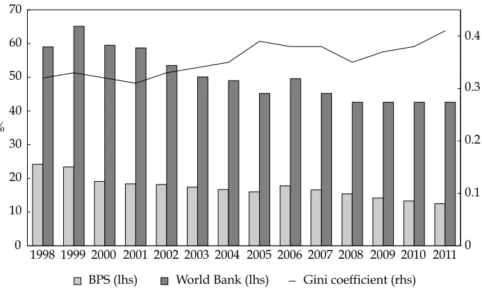
BPS publishes the Gini coeficient only periodically, but Cameron (2002) lists the Gini coeficient from both Asra (2000) and Booth (2000) during 1964–99, in which it ranges from 0.32 to 0.38. Figure 1 shows that the increase in Indone

-sia’s oficial Gini coeficient after 2001 was not accompanied by an increase in the

number of poor. According to data from both BPS and the World Bank, whose

(3)

FIGURE 1 Indonesia’s Poverty Rate and the Gini Coeficient, 1998–2011a

!

a_{Includes predicted igures for 2009–11 for the Gini coeficient and the poverty rate based on the} World Bank deinitions. See the text for the BPS and World Bank deinitions of poverty.

Source: Ministry of Finance (2012).

average poverty line for developing countries sits at $2 per capita per day, or $60 per month (World Bank 2009), the number of poor in Indonesia has decreased

since 1999 (igure 1). The data suggest that the increase in income at the bottom of

the distribution is less than the increase at the top of the distribution, indicating

a wider dispersion. However, annual increases of around 5% in average income during 1998–2008 reduced the number of poor in Indonesia by around 8% each

year.1

This paper evaluates different measurements of household income distribution

in Indonesia. Previous studies (Cameron 2002; Lanjouw et al. 2002; Chung 2004)2

have used household consumption to measure income inequality, because consumption data are generally more reliable than income data and are a better

indicator of a household’s permanent income (Deaton 1997). Here, we evaluate

income inequality by using household income (comprising both market and non-market income) to strengthen the literature on income inequality in Indonesia.

In a country such as Indonesia, market income may not capture all of the components of ‘actual’ income, which includes, for example, consumption of own

1 Economic growth’s role in reducing poverty has been demonstrated elsewhere. Cameron (2002) found that Indonesia’s rapid rate of average real economic growth (7.1% per annum) during 1968–97 did not change inequality levels markedly. Fields et al. (2003) demonstrated that in Indonesia, South Africa, Spain and Venezuela, those with the lowest average household incomes enjoyed the most favourable income changes during the 1990s. 2 Leigh and Van der Eng (2010) compare expenditure- and income-based Gini ratios for 1982–2004 and then use the household income data to analyse trends in top income.

(4)

Towards a better measure of income inequality in Indonesia 105

production (a household’s consumption of the goods it produces itself, such as vegetables) and income in kind (income received in such forms as gifts, money

transfers, company cars, meals and barter trade). Kusnic and Davanco (1986)

maintain that in developed countries, households once produced many goods and services now supplied by the market. In developing countries, traditional measures that exclude household production under-estimate the ‘actual’ income of the poor. Similarly, expenditure data that include only market purchases will

also signiicantly under-estimate ‘actual’ income and consumption.

This paper uses the household characteristics (module) and individual charac-teristics (core) of the 2009 National Socio-Economic Survey (Susenas) to calculate income distribution and adjusted income per capita for market income and actual income. The term ‘actual income’ refers to all market and non-market income that affects household living standards. Actual income comprises household market

income, consumption of own production and income in kind. Evers (1981) con -cluded that, at the time, subsistence production was the third most important sector in the Indonesian economy, behind the formal and informal sectors. Today, subsistence-oriented monoculture production in agriculture, for example, is as important as ever, yet consumption of own production and income in kind have not contributed to analyses of income distribution in Indonesia.

The Susenas core and module data allow us to incorporate personal information, such as the age of each household member, in our analysis. We have taken household market income, that is, income after income tax, from the 2009 Susenas. Non-market income also includes consumption of own production, income in kind, and other income calculated using the household expenditure module and imputing non-market income to households.

The irst and second sections of this paper explain, respectively, our methodology and use of data. The third section discusses our indings, and the fourth section

concludes.

METHODOLOGY

This paper calculates household market income using the household income

reported in the 2009 Susenas. BPS (2009) deines market income as:

• wages and salaries, including money, goods and services;

• business income, including food agriculture, other agriculture (such as

non-food agriculture, farming, isheries, forestry and hunting) and non-agriculture

(such as industry, trade, transportation, service, construction and mining); and

• non-business income, including income from rent and other assets (such as interest, dividends, royalties and land rents).

Our analysis of Susenas data from block 5 (household income and expendi -ture) revealed that survey participants rarely include goods and services (that is,

their non-market income) in their responses to questions about their income. For example, the data contains gaps between market income plus inancial income

and household consumption minus own production, and between total house-hold income and total househouse-hold expenditure. Respondents rarely include their non-market income in Susenas, but they often include all of their consumption

expenditure; non-market income should be added to the income they receive

(5)

from wages and salaries in kind, gifts, or other unidentiied income. Susenas also

captures data for household consumption from the week of the survey, and asks, for example, ‘how many eggs did you eat in the last week?’. Participants tend to report all they eat, even though they may not have purchased all of it (it may have been provided by employers, for example, or obtained through bartering).

The formula for income in kind is as follows:

Yk

i=

(

Exi−Yni−Coi−Fi

)

i₌i

n

∑ (1)

where Yk_i is the income in kind of household i; Ex_i is the total expenditure of household i, including inancial expenditure (such as savings, debt payments, insurance premiums and loans); Yn_i is the net income of household i; Co_i is the consumption of own production of household i; and F_i is the inancial income of

household i (such as withdrawals, credit payments, insurance claims and

borrow-ings). We introduce inancial income and inancial expenditure to capture saving and borrowing’s role in inancing expenditure. Here, income in kind is the part of household total expenditure that is not inanced by, for example, market income, inancial income or consumption of own production.

We add consumption of own production to market income, because this

consumption can signiicantly increase a household’s standard of living. We

combine household income data and household expenditure data from Susenas, to analyse the quantity and value of each household’s consumption of own production. BPS (2009) calculates the value of consumption of own production based on the relevant region’s market price and adds it to consumption expenditure.

Previous studies (Cameron 2000; Leigh and Van der Eng 2010) have calculated Indonesia’s Gini coeficient using food and non-food consumption (Susenas

block 4.3), which is similar to BPS’s method. These studies equate household

consumption to household expenditure, but, as our analysis of Susenas block 5

reveals, household consumption differs from household expenditure. We use total household expenditure, which captures income in kind and unreported income (the difference between total expenditure and total income).

Before calculating the effect of total household expenditure’s on income distribution, we divided both categories of income, that is, market income and actual income, by equivalence scales, to account for household size and to determine adjusted per capita income. Equivalence scales compare the income

levels of households of different size and composition – a larger household

needs to have a higher level of income to achieve the same standard of living as

a smaller household (ABS 2007). Such scales recognise that the economic needs

of additional adults and children in households are not equal to the economic

needs of the irst adult and child. Many elements determine the economic need

of each household member. Working adults, for example, incur transportation costs, and older children cost more to raise than young children. The most

common equivalence scale is that modiied by the OECD (Hagenaars, de Vos and

Zaidi 1994). However, Ree, Alessie and Pradhan (2013) argue that this scale is not appropriate in Indonesia, in which households spend, on average, a larger fraction of their total budget on food than do households in OECD countries.

(6)

To simplify the measurement of adjusted per capita income, we use an equivalence scale that assigns different weights to each household member: the

irst adult is assigned 1 point, each additional person above 15 years is assigned 0.5 points, the irst child under 15 years is assigned 0.5 points and each additional child under 15 years is assigned 0.35 points (Ree, Alessie and Pradhan 2013). Following the approach of Kim et al. (2006), we deine children as those under 15 years and adults as those over 15 years. The formula for adjusted per capita

income is as follows: variable that takes the value of 1 or 0, indicating whether there is at least one adult in the household, i; n_i is the number of adults in the household; a_ic is a dummy variable indicating whether there is at least one child in the household; and n_ic is the number of children in the household.

We used four ways of calculating the effects of all income categories on income distribution:

• Nominal and share terms: In nominal terms, we used US dollar values, to enable international comparisons and to use PPP to account for price differences. The

average PPP exchange rate in 2008 was Rp 5,410 = $1. Price differences across

regions are important, especially in Indonesia, but they are hard to measure,

since only inlation rates (and not price indexes) are available for each region.

In share terms, we divided the income of each group by the aggregate income of the population.

• Income groups: We ranked the household samples from the lowest to the highest, on the basis of their adjusted income, and then divided them into deciles. Each

decile contained 5,754,867 weighted households. Comparing the share of these

income deciles gives the dispersion of household income.

• Gini coeficient and percentile ratios: The Gini coeficient is a well-known indicator of income inequality. The formula is as follows:

where Y_iand Y_jare individual incomes with a mean of Ŷ, and where n is the

total number of observations (Rosen and Gayer 2008). A higher igure indicates

a higher level of income inequality.

• Decile earnings compared with median earnings: Comparing the earnings of the lowest and highest deciles relative to median earnings

gives the dispersion of earning (Lewis et al. 2010). The formula is:

where D is the dispersion of earning, P10_{is the lowest percentile of earnings,}

P50_{is median earnings and}_P90_{is the highest percentile of earnings.}

Gini= i=1

(7)

DATA

Susenas collects data annually from a sample of households that are individu-ally weighted to represent the Indonesian population. The Susenas core collects individual and household characteristics, such as age, employment status, health, education level and housing type, whereas the Susenas module collects

informa-tion on speciic topics, such as household consumpinforma-tion and expenditure, in

three-year cycles. At the time of our research, the most recent Susenas core data were for

2008 (2009 publication) and were collected from 1,142,675 individuals and 282,387 households; the latest module data on consumption and expenditure were also for 2008, and were collected from the same number of households. To capture

a complete set of information on households and their individuals’ characteris-tics, consumption patterns, per capita expenditure and income distribution, we

merged Susenas core and module data – the irst such merging of individual and

household data from Susenas.3

One problem of using Susenas data is the potential under-representation of

the very wealthy and the very poor (Cameron 2002); the former tend to refuse to respond to the questions of the BPS oficers, and it is hard to collect data from the

latter. As in the household surveys of some other countries, the highest earners

– especially the top 10% – receive only limited statistical coverage (Deaton 1997).

This gap in Susenas data is borne out by the substantial discrepancy between total household expenditure estimated from Susenas and the total private consumption

component of GDP (Leigh and Van der Eng 2010). With this in mind, the results

of this paper should be considered as representing all but the very poorest and richest households in Indonesia.

FINDINGS AND DISCUSSION

We calculated three types of adjusted income for comparison: per capita income;

adjusted per capita income, based on the equivalence scale of Ree, Alessie and

Pradhan (2013); and adjusted per capita income based on the OECD equivalence

scale. Our results differ slightly for certain household types by income quintile,

but they were not signiicantly altered by our choice of method. To capture

the impact of household size, then, we present only those results based on the equivalence scale above.

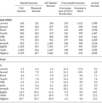
Table 1 shows the distribution of adjusted per capita market, non-market and actual income for each decile. It shows that the dispersion of actual income is greatly reduced after adding income in kind and consumption of own production

to all market income, which comprises net income and inancial income. The proportion of income by household in the highest decile is 32.0% for market income and 22.2% for actual income; in the lowest decile, these proportions are 2.2% and 8.1% respectively. Actual income’s share in the lowest decile, by market income, is higher than that in the second to fourth deciles. The poorest beneit more from

non-market income than those in the second to fourth deciles. The dispersion of income in kind and consumption of own production for each household group is fairly systematic in reducing the level of inequality between income groups.

3 Leigh and Van der Eng (2010) summed individual data to household levels for 1999 and 2002.

(8)

Income in kind and consumption of own production are important for all income groups, including the richest households.

Actual income is signiicantly higher than all market income in all deciles. For example, in the lowest decile, actual income, $1,590, is more than six times all market income, $254. For households in the lowest decile, non-market income

plays a big role in increasing the standard of living. Even for the highest decile,

actual income is around 20% higher than all market income. There is far less inequality in actual income than in market income. This inding is in line with those of Evers (1981) and Ravallion and Dearden (1988). Evers (1981) inds that

subsistence production plays a major role in the household economy in Indonesia,

particularly for the poor. Ravallion and Dearden (1988) mention the signiicant role

of ‘moral economy’ in Java, since there is no social-security system in Indonesia. Moral economy is the transfer payment of money or goods from rich to poor households.

TABLE 1 Household Per Capita Income in 2008, by Decile

Market Income All Market

a_{PPP$ = purchasing-power-parity dollars.}

Source: Authors’ calculations based on data from the 2009 Susenas module.

(9)

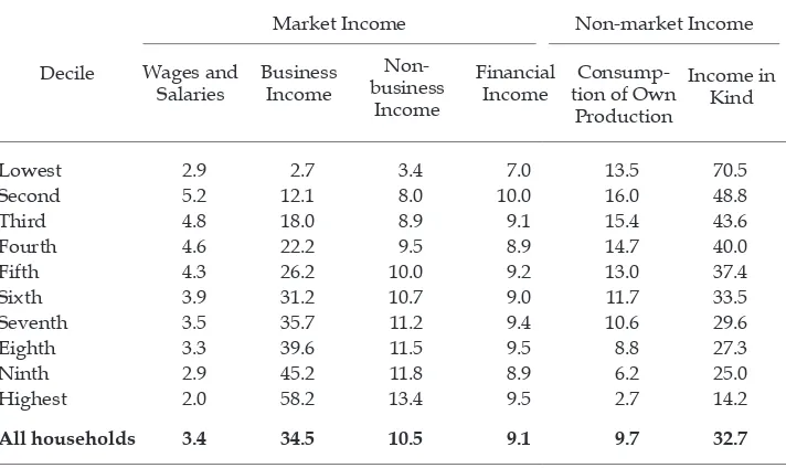
Table 2 shows the sources of per capita income in each household group. In the lowest and second deciles, the largest source of income is income in kind and

consumption of own production. These indings have implications for taxation. For households in these deciles, most of their income is non-market income;

low-income households pay less low-income tax than other deciles. In the third to sixth deciles, most income comes from income in kind and then from business income. Taxes are paid on business income but not on income in kind. In the seventh to highest deciles, most income comes from business income and then from income in kind. The amount of tax paid is higher than that paid by households in other deciles, because most of the income is from business income. Even those households in the highest deciles have some consumption of own production.

The share of inancial income in adjusted per capita household income is simi

-lar for all deciles. We can speculate that most inancial income in the lowest deciles

comes from borrowing and in the highest deciles from saving.

Income inequality

Two of the most common ways of measuring income inequality are the Gini

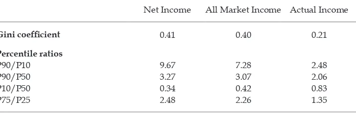
coeficient and relative percentiles. Table 3 shows that the Gini coeficient for

adjusted per capita net income is 0.41. Within a range of 0 to 1, a value of 0 means

perfectly equal and 1 means perfectly unequal (Lewis et al. 2010). Adding inancial income to net income reduces the Gini coeficient to 0.40, indicating a lower level

of inequality. When income in kind and consumption of own production are also

included, the Gini coeficient reduces further, to 0.21 (table 3). Non-market income

improves the standard of living of the lowest income group most, which also

reduces income inequality. If we compare this Gini coeficient with that of BPS, TABLE 2 Sources of Adjusted Household Actual Per Capita Income in 2008

(%)

(10)

the level of income inequality in Indonesia is much lower than the oficial level: using expenditure data for individual households, we calculate a Gini coeficient of 0.31, which, based on grouped data, is comparable with BPS’s estimate of 0.37.

This alternative calculation of the Gini coeficient points to a lower level of

income dispersion than that measured by BPS and the World Bank, as measured

by relative percentiles. The ratio of the lowest 10% to the median of income changes from 0.34 to 0.83 – that is, the income of the lowest decile increases from 34% of the median income to 83%. The ratio of the highest 10% of incomes to the median of income changes from 3.27 to 2.06. This means that the market income

of the highest-earning households is around 3.3 times the median income, but this falls to around 2.1 times when actual income is used.

CONCLUSION

Indonesia’s poverty rate has fallen rapidly since 2000 but is still higher than

that of most of its neighbours. In 2008, the proportion of the population living

on less than $2 a day (at 2005 international prices) in Indonesia was 54.4%, compared with 53.3% in Cambodia and 43.4% in Vietnam (World Bank 2012). To reduce poverty and improve income distribution, it is necessary to start with an

appropriate measure of income inequality. In this paper, we use a broad deinition

of income for this purpose, and include both market and non-market income in our calculations of total household income. All income groups in Indonesia earn non-market income, but households in the lowest income deciles have a larger proportion of non-market income than the highest income groups.

Our results suggest that measuring income inequality in Indonesia without assessing non-market income gives misleading results, and that non-market

income contributes signiicantly to lower levels of income inequality. The

dispersion of actual income is more balanced after adding income in kind and consumption of own production to income calculations, because both components have the potential to increase the income of the lowest- and middle-income

groups. Calculating the Gini coeficient and dispersion of income using market income alone – the method used in most developed countries – is not suitable for

Indonesia.

TABLE 3 Inequality Measures of Adjusted Per Capita Income in 2008

Net Income All Market Income Actual Income

Gini coeficient 0.41 0.40 0.21

Percentile ratios

P90/P10 9.67 7.28 2.48

P90/P50 3.27 3.07 2.06

P10/P50 0.34 0.42 0.83

P75/P25 2.48 2.26 1.35

(11)

REFERENCES

ABS (Australian Bureau of Statistics) (2007) Government Beneit, Taxes and Household Income, Cat. no. 6537.0, Canberra.

Asra, A. (2000) ‘Poverty and inequality in Indonesia: estimates, decomposition and key issues’, Journal of the Asia Paciic Economy 51 (1–2): 91–111.

Booth, A. (2000) ‘Poverty and inequality in the Soeharto era: an assessment’, Bulletin of Indonesian Economic Studies 36 (1): 73–104.

BPS (Badan Pusat Statistik) (2009) Survei Sosial Ekonomi Nasional (National Socio- economic Survey, Susenas), Republic of Indonesia, Jakarta.

BPS (Badan Pusat Statistik) (2010) Statistik Indonesia (Statistical Yearbook of Indonesia), Republic of Indonesia, Jakarta.

Cameron, L. (2000) ‘Poverty and inequality in Java: examining the impact of the chang -ing age, educational and industrial structure’, Journal of Development Economics 62 (1): 149–180.

Cameron, L. (2002) ‘Growth with or without equity? The distributional impact of Indone -sian development’, Asian-Paciic Economic Literature 16 (2): 1–17.

Chung, W. (2004) ‘Income inequality and health: evidence from Indonesia’, Centre for Labour Market Research Discussion Paper Series 4 (3): 1–12.

Deaton, A. (1997) The Analysis of Household Surveys: A Microeconomic Approach to Develop-ment Policy, World Bank, Johns Hopkins University Press, Maryland.

Evers, H.D. (1981) ‘The contribution of urban subsistence production to incomes in Jakarta’, Bulletin of Indonesian Economic Studies 17 (2): 89–96.

Fields, G.S., Cichello, P.L., Freije, S., Menendez, M, and Newhouse, D. (2003) ‘For richer or for poorer? Evidence from Indonesia, South Africa, Spain and Venezuela’, Journal of Economic Inequality 1: 67–99.

Hagenaars, A., de Vos, K. and Zaidi, M.A. (1994) Poverty Statistics in the Late 1980s: Research Based on Micro Data, Ofice for Oficial Publications of the European Communities, Lux -embourg.

Kim, J., Engelhardt, H., Prskawetz, A. and Aaassve, A. (2006) Does Fertility Decrease the Welfare of Households? An Analysis of Poverty Dynamics and Fertility in Indonesia, Vienna Institute of Demography, Vienna.

Kusnic, M. and Davanco, J. (1986) ‘Accounting for non-market activities in the distribution of income: an empirical investigation’, Journal of Development Economics 21 (2): 211–27. Lanjouw, P., Pradhan, M., Saadah, F., Sayed, H. and Sparrow, R. (2002) ‘Poverty, education

and health in Indonesia: who beneits from public spending?’, in Education and Health Expenditures, and Development: The Cases of Indonesia and Peru, ed. C. Morrisson, OECD Development Centre, Paris: 17–78.

Leigh, A. and Van der Eng, P. (2010) ‘Top incomes in Indonesia, 1920–2004’, in Top Income: A Global Perspective, eds A.B. Atkinson and T. Piketty, Oxford University Press, Oxford: 171–219.

Lewis, P., Garnett, A., Treadgold, M. and Hawtrey, K. (2010) The Australian Economy: Your Guide, Pearson Education Australia, Sydney.

Ministry of Finance (2012) Buku Saku APBN dan Indikator Ekonomi (Handbook of Budget and Economic Indicators), Republic of Indonesia, Jakarta.

Ravallion, M. and Dearden, L. (1988) ‘Social security in a “moral economy”: an empirical analysis for Java’, Review of Economics and Statistics 70 (1): 36–44.

Ree, J., Alessie, R. and Pradhan, M. (2013) ‘The price and utility dependence of equivalence scales: evidence from Indonesia’, Journal of Public Economics 97: 272–81.

Rosen, H.S. and Gayer, T. (2008) Public Finance, McGraw-Hill, New York.

World Bank (2009) ‘Indonesian economic indicators’, Country Report, World Bank, Wash-ington DC.

World Bank (2012), ‘Poverty headcount ratio at $2 a day (PPP) (% of population)’, avail -able at <http://data.worldbank.org/indicator/SI.POV.2DAY/countries/1W?display= default>.