Full Terms & Conditions of access and use can be found at
http://www.tandfonline.com/action/journalInformation?journalCode=ubes20
Download by: [Universitas Maritim Raja Ali Haji] Date: 12 January 2016, At: 17:42
Journal of Business & Economic Statistics
ISSN: 0735-0015 (Print) 1537-2707 (Online) Journal homepage: http://www.tandfonline.com/loi/ubes20
A Comparison of the Real-Time Performance of
Business Cycle Dating Methods
Marcelle Chauvet & Jeremy Piger
To cite this article: Marcelle Chauvet & Jeremy Piger (2008) A Comparison of the Real-Time Performance of Business Cycle Dating Methods, Journal of Business & Economic Statistics, 26:1, 42-49, DOI: 10.1198/073500107000000296
To link to this article: http://dx.doi.org/10.1198/073500107000000296
Published online: 01 Jan 2012.
Submit your article to this journal
Article views: 226
View related articles
A Comparison of the Real-Time Performance of
Business Cycle Dating Methods
Marcelle C
HAUVETDepartment of Economics, University of California, Riverside, CA 92521 (chauvet@ucr.edu)
Jeremy P
IGERDepartment of Economics, University of Oregon, Eugene, OR 97403 (jpiger@uoregon.edu)
We evaluate the ability of formal rules to establish U.S. business cycle turning point dates in real time. We consider two approaches, a nonparametric algorithm and a parametric Markov-switching dynamic-factor model. Using a new “real-time” dataset of coincident monthly variables, we find that both approaches would have accurately identified the NBER business cycle chronology had they been in use over the past 30 years, with the Markov-switching model most closely matching the NBER dates. Further, both ap-proaches, and particularly the Markov-switching model, yielded significant improvement over the NBER in the speed with which business cycle troughs were identified.
KEY WORDS: Dynamic-factor model; Markov-switching; Recession; Turning point; Vintage data.
1. INTRODUCTION
There is a long tradition in business cycle analysis of sepa-rating periods in which there is broad economic growth, called expansions, from periods of broad economic contraction, called recessions. Understanding these phases and the transitions be-tween them has been the focus of much macroeconomic re-search over the past century. In the United States, the National Bureau of Economic Research (NBER) establishes a chronol-ogy of “turning point” dates at which the shifts between expan-sion and recesexpan-sion phases occur. These dates are nearly univer-sally used in work requiring a definition of U.S. business cycle phases. Since 1978, business cycle dates have been established in real time by the NBER’s Business Cycle Dating Committee, which is currently composed of seven academic economists.
The NBER’s announcements garner considerable publicity. Given this prominence, it is not surprising that the business cy-cle dating methodology of the NBER has received some crit-icism. For example, because the NBER’s decisions represent the consensus of individuals who likely bring differing tech-niques to bear on the question of when turning points occur, the dating methodology is charged as being neither transparent nor reproducible. Also, the NBER has been hesitant to revise busi-ness cycle turning point dates, despite the fact that economic data are revised substantially. Finally, the NBER business cycle peak and trough dates are often determined with a substantial lag. For example, the March 1991 and November 2001 business cycle troughs were not announced by the NBER until nearly two years after the fact.
An alternative to the NBER procedures is to use formal rules to date business cycle turning points. Such rules immediately address the first two criticisms above. That is, given that the rules take the form of a formal algorithm or statistical model ap-plied to data, they are both transparent and reproducible. Also, because the rules can be applied to revised data, they provide a straightforward approach to revision of business cycle dates. In this article we evaluate whether such rules can also address the third critique. That is, do these rules provide more timely identification of business cycle dates? Of course, any gain in timeliness must be weighed against any loss of accuracy in es-tablishing the dates. To measure accuracy, we take it as given
that the NBER established the correct turning point dates in real time, thus making the NBER chronology the standard for accu-racy.
Why are we interested in the speed with which business cycle turning points can be identified? The NBER is likely more con-cerned with establishing the correct turning point dates than es-tablishing these dates quickly, which breeds additional caution. This caution comes at a low cost if the primary objective is to provide a historical record of business cycle phases. However, as there is substantial evidence that interesting economic dy-namics and relationships vary over business cycle phases, eco-nomic agents are likely also interested in real-time monitoring of whether a new phase shift has occurred. In this article we provide some formal evidence regarding the speed with which such real-time monitoring can reveal a new turning point in eco-nomic activity.
We compare two popular business cycle dating methods, both of which are multivariate in that they use information from many time series to establish business cycle dates. The first is a nonparametric algorithm, developed and discussed in Harding and Pagan (2006) and denoted MHP, for multivariate Harding– Pagan, hereafter. The MHP algorithm proceeds by first identi-fying turning points as local minima and maxima in the level of individual time series. Next, economy-wide turning points are established by finding dates that minimize a measure of the average distance between that date and the turning points in in-dividual series.
The second approach is a parametric dynamic factor time se-ries model that captures expansion and recession phases as un-observed regime shifts in the mean of the common factor. The unobserved state variable controlling the regime shifts is mod-eled as following a Markov process as in Hamilton (1989). This Markov-switching dynamic factor model (DFMS), as devel-oped in Chauvet (1998), produces a probability that the econ-omy is in an expansion or a recession at any point in time. These probabilities can then be used to establish turning point dates
© 2008 American Statistical Association Journal of Business & Economic Statistics January 2008, Vol. 26, No. 1 DOI 10.1198/073500107000000296 42
Chauvet and Piger: Business Cycle Dating Methods 43
using a rule for converting probabilities into a zero/one variable defining which regime the economy is in at any particular time. We apply these two approaches to a new “real-time” dataset of the four coincident economic variables highlighted by the NBER in establishing turning point dates: (1) nonfarm payroll employment, (2) industrial production, (3) real manufacturing and trade sales, and (4) real personal income excluding transfer payments. In particular, the dating methods are applied as if an analyst had been using them to search for new turning points each month beginning in November 1976, where the data used is the vintage that would have been available in that month. This real-time dataset was collected for this article and has not yet been applied in any other analysis.
The results of this exercise suggest that both approaches are capable of identifying turning points in real time with reason-able accuracy. That is, the first time these methods declare a turning point, the chosen date is usually close to that estab-lished by the NBER. The most accurate performance is given by the DFMS model, which provides turning point dates in real time that are usually within one month, and never more than two months, from the corresponding NBER date. Both meth-ods achieve this performance with no instances of “false posi-tives,” or turning point dates that were established in real time, but did not correspond to a NBER turning point date. Further, both approaches improve significantly over the NBER in the speed at which business cycle troughs are identified. In par-ticular, the DFMS model would have identified the four busi-ness cycle troughs in the sample an average of 249 days, or roughly 8 months, ahead of the NBER announcement, whereas the MHP algorithm would have led by an average of 166 days, or about 5.5 months. However, neither approach provides a cor-responding improvement in the speed with which business cy-cle peaks are identified. Overall, these results suggest that for-mal dating rules are a potentially useful tool to be used for real-time monitoring of business cycle phase shifts.
Our article makes several contributions to an existing liter-ature on this topic. Layton (1996) evaluated the performance of Markov-switching models of the U.S. coincident index for establishing business cycle turning points. Layton used a “pseudo” real-time analysis in which fully revised data are used in recursive estimations to evaluate the real-time perfor-mance of the business cycle dating algorithm. The new real-time dataset we use here provides a more realistic assessment of how the dating rules would have performed, as it does not as-sume knowledge of data revisions that were not available at the time the rule would have been used. Chauvet and Piger (2003) used real-time data to evaluate the business cycle dating perfor-mance of univariate Markov-switching models of employment and real GDP, and Chauvet and Hamilton (2006) did a simi-lar exercise for multivariate Markov-switching models. These articles consider only Markov-switching models, whereas here we compare Markov-switching models to nonparametric algo-rithms, which have a long history in dating business cycles. Harding and Pagan (2003) also provided some comparison of univariate versions of the dating rules considered here. How-ever, this comparison does not consider multivariate methods or the real-time performance of the methods.
In the next section we discuss the two approaches used to establish business cycle turning points in more detail. Section 3
describes the real-time dataset. Section 4 discusses the real-time performance of the models for dating turning points in the busi-ness cycle. Section 5 concludes.
2. DESCRIPTION OF THE BUSINESS CYCLE DATING METHODS
The NBER dates a turning point in the business cycle when a consensus of the Business Cycle Dating Committee that a turning point has occurred is reached. Although each Commit-tee member likely brings different techniques to bear on this question, the decision is framed by the working definition of a business cycle provided by Arthur Burns and Wesley Mitchell (1946, p. 3):
Business cycles are a type of fluctuation found in the aggregate economic ac-tivity of nations that organize their work mainly in business enterprises: a cycle consists of expansions occurring at about the same time in many economic activities, followed by similarly general recessions, contractions and revivals which merge into the expansion phase of the next cycle.
Fundamental to this definition is the idea that business cy-cles can be divided into distinct phases. In particular, expan-sion phases are periods when economic activity tends to trend up, whereas recession phases are periods when economic activ-ity tends to trend down. In addition, the definition stresses that these phases are observed in many economic activities, a con-cept typically referred to as comovement. In practice, to date the shift from an expansion phase to a recession phase, or a busi-ness cycle peak, the NBER looks for clustering in the shifts of a broad range of series from a regime of upward trend to a regime of downward trend. The converse exercise is performed to date the shift back to an expansion phase, or a business cycle trough. Four monthly series are prominently featured by the NBER in their decisions: employment, industrial production, real manu-facturing and trade sales, and real personal income excluding transfer payments.
The two business cycle dating methods that we consider in this article represent attempts to operationalize the above defin-ition into formal algorithms and statistical models. We turn now to a more detailed discussion of both methods.
2.1 Harding and Pagan (2006) Algorithm
Based on relatively informal descriptions of NBER proce-dures laid out in Boehm and Moore (1984), Harding and Pa-gan (2006) developed a formal algorithm whereby a common set of turning points can be extracted from a group of individ-ual time series. The algorithm is described in detail in Hard-ing and Pagan (2006), and we provide only a brief summary here for a group of monthly time series. Before using the al-gorithm, we need to first extract turning point dates for each of the time series, indexed by i=1, . . . ,I. Here we employ the commonly used algorithm of Bry and Boschan (1971) for this purpose, which, roughly speaking, identifies turning points as local minima and maxima in the path of each time se-ries. To implement the Bry–Boschan algorithm, we use Gauss code created for Watson (1994). Once the Bry–Boschan algo-rithm has been applied to each time series, we have a set ofI
turning point histories, labeled{P1,P2, . . . ,PI}for peaks and
{T1,T2, . . . ,TI}for troughs, wherePiandTiare vectors of
turn-ing point dates for time seriesi. The contribution of the Harding
and Pagan algorithm is to consolidate these individual peak and trough dates into a single set of common turning point dates. To do this, Harding and Pagan defined variablesDPitandDTit,
which record the distance in months between monthtand the nearest entry in Pi for DPit and Ti for DTit. For example, if
Pi =(20,40,60) and t=45, then DPit =5. For each value
of t, we then form DPt and DTt as the median across the I
time series, that is, DPt =median(DP1t,DP2t, . . . ,DPIt)and
DTt=median(DT1t,DT2t, . . . ,DTIt). Harding and Pagan then
defined the common peak and trough dates as local minima in
DPt andDTt. Formally, a common peak or trough is defined
at month t ifDPt or DTt is a minimum value in a 31-month
window centered at time t, that is, fromt−15 to t+15. In practice, these local minimum values may not be unique, and it may be necessary to break ties. To do so, Harding and Pagan considered higher percentiles than the median until a unique local minimum was found.
Finally, once the candidate set of common turning points has been obtained, two censoring procedures are applied. First, for a candidate common peak (trough) to be retained at timet, the median distance to individual turning point dates, that is, the value ofDPt(DTt), must not be larger than 15 months. Second,
turning points are recombined so that they alternate between peaks and troughs.
2.2 Dynamic Factor Markov-Switching Model
As discussed earlier, the NBER definition of a business cycle places heavy emphasis on regime shifts in economic activity. Given this, the Markov-switching model of Hamilton (1989), which endogenously estimates the timing of regime shifts in the parameters of a time series model, seems well suited for the task of modeling business cycle phase shifts. In addition, the NBER definition stresses the importance of comovement among many economic variables. This feature of the business cycle is often captured using the dynamic common factor model of Stock and Watson (1989, 1991).
Chauvet (1998) combined the dynamic-factor and Markov-switching frameworks to create a statistical model capturing both regime shifts and comovement. Specifically, definingYit
as the log level of theith time series, andy∗it=yit− ¯yi as the
demeaned first difference ofYit, the DFMS model has the form ⎡
That is, the demeaned first difference of each series is made up of a component common to each series, given by the dynamic factorct, and a component idiosyncratic to each series, given
byeit. The common component is assumed to follow a
station-ary autoregressive process:
φ (L)(ct−μSt)=εt, (2)
whereεt is a normally distributed random variable with mean
zero and variance set equal to unity for identification purposes, andφ (L)is a lag polynomial with all roots outside of the unit circle. The common component is assumed to have a switch-ing mean, given by μSt =μ0+μ1St, where St= {0,1}is a
state variable that indexes the regime andμ1<0 for
normal-ization purposes. The state variable is unobserved, but is as-sumed to follow a Markov process with transition probabilities
P(St=1|St−1=1)=p andP(St =0|St−1=0)=q. Finally,
each idiosyncratic component is assumed to follow a stationary autoregressive process:
θi(L)eit=ωit, (3)
whereθi(L)is a lag polynomial with all roots outside the unit
circle.
Chauvet (1998) estimated the DFMS model for U.S. monthly data on nonfarm payroll employment, industrial production, real manufacturing and trade sales, and real personal income excluding transfer payments. The model produced estimated probabilities of the regime at time t conditional on the data, denotedP(St=1|T), that closely matched NBER expansion
and recession episodes. That is,P(St=1|T)was high during
recessions and low during expansions.
In this article, we use the DFMS model to obtain recession probabilities in real time. Also, because we are interested in obtaining specific turning point dates, we will require a rule to convert the recession probabilities into a zero/one variable that defines whether the economy is in an expansion or a re-cession regime at time t. Here, we take a conservative, two-step approach, which we outline for a business cycle peak. In the first step, we require that the probability of recession move from below to above 80% and remain above 80% for three consecutive months before a new recession phase is iden-tified. That is, we require thatP(St+k=1|T)≥.8, fork=0
to 2 and P(St−1=1|T) < .8. In the second step, the first
month of this recession phase is identified as the first month prior to montht for which the probability of recession moves above 50%. That is, we find the smallest value ofqfor which
P(St−q−1=1|T) < .50 andP(St−q=1|T)≥.50. The peak
date for this recession phase is then established as the last month of the previous expansion phase, or montht−q−1. An anal-ogous procedure, with the 80% threshold replaced by 20%, is used to establish business cycle troughs.
To estimate the parameters of the DFMS model, as well as the recession probabilities, we use the Bayesian Gibbs Sam-pling approach described in Kim and Nelson (1998). The Gibbs Sampler produces a posterior distribution for St conditional
on the data, T, the mean of which corresponds to the
re-cession probabilityP(St=1|T). These probabilities are then
used to obtain business cycle turning point dates. Priors for the Bayesian estimation are quite diffuse, and match those used in Kim and Nelson (1998). We set the lag order of each autore-gressive polynomial,φ (L)and θi(L), equal to 2. This choice
of lag order is based on specification tests reported in the stud-ies of Stock and Watson (1991), Chauvet (1998), and Kim and Nelson (1998), each of which suggested that 2 lags is sufficient for dynamic-factor models of the four coincident variables we consider here.
3. REAL–TIME DATASET
In this section we describe the real-time dataset. We have compiled real-time data on four coincident variables: (1) non-farm payroll employment (EMP), (2) industrial production (IP),
Chauvet and Piger: Business Cycle Dating Methods 45
(3) real manufacturing and trade sales (MTS), and (4) real per-sonal income excluding transfer payments (PIX). These are the four monthly variables highlighted by the NBER in establish-ing turnestablish-ing point dates. We have collected realizations, or vin-tages, of these time series as they would have appeared at the end of each month from November 1976 to June 2006. For each vintage from November 1976 to January 1996, the sample col-lected begins in January 1959 and ends with the most recent data available for that vintage. For each vintage from February 1996 to June 2006, the sample begins in January 1967. For the series EMP, IP, and PIX, data are released for monthtin month
t+1. Thus, for these variables the sample ends in monthR−1 for vintageR. For MTS, data are released for monthtin month
t+2. Thus, for this variable the sample ends in monthR−2 for vintageR. We obtained the EMP and IP data series from the Federal Reserve Bank of Philadelphia real-time data archive de-scribed in Croushore and Stark (2001). Data for PIX and MTS were hand-collected as part of a larger real-time data collection project at the Federal Reserve Bank of St. Louis. This dataset is new and has not yet been used in any other applications. The Appendix provides more detail on the sources used to collect the PIX and MTS series.
4. PERFORMANCE OF THE BUSINESS CYCLE
DATING METHODS
4.1 Description of Real-Time Simulation Exercise
To assess the real-time performance of the two business cy-cle dating methods described in Section 2, we apply these tech-niques to the real-time dataset described in Section 3. We as-sume that an analyst applies the business cycle dating methods on the final day of each month, which is soon after the release of MTS data for that monthly vintage. Thus, for each monthly vintageR, we create a monthly dataset of EMP, IP, MTS, and PIX that would have been available at the end of monthR. The final month of data included in this dataset is determined by the series with the least amount of data available at vintageR. As discussed in Section 3, this final data point is monthR−2, which is the last month for which data are available for MTS. For each vintageR, the MHP algorithm and DFMS model are applied to the dataset, and a chronology of turning point dates determined. We will be particularly interested in evidence of new turning points revealed toward the end of the sample at vintageR.
The choice to restrict the entire dataset by the series with the least data available at vintageR is a conservative assess-ment of the information available to the analyst. Alternatively, we could have included the monthR−1 data for EMP, IP, and
PIX in conjunction with a forecast for monthR−1 MTS data. Although potentially fruitful, we chose not to pursue this ap-proach here for two reasons. First of all, as will be seen later, the performance of the business cycle dating methods applied to the restricted dataset is already quite good, thus demonstrating the potential benefits of their use. Second, it is not clear that the additional information for EMP, IP, and PIX would necessarily improve the performance of the dating methods, as revisions from the first to the second release of these monthly data series, particularly EMP and IP, are often very large.
Finally, it should be noted that there are two elements of this experiment that are not “real time” in nature. First of all, whereas the parameters of the DFMS model are re-estimated at each vintage, the lag orders for the DFMS model specifica-tion remain fixed across vintages. The chosen lag orders were based on specification tests conducted in prior studies, namely, Stock and Watson (1991), Chauvet (1998), and Kim and Nel-son (1998). However, because all of these studies used data not available at the earlier vintages in our dataset, for each of these earlier vintages the chosen lag orders are based on data that would not have been available at that vintage. Second, the rule used to convert recession probabilities obtained from the DFMS model into turning point dates was selected with knowl-edge of the estimated recession probabilities obtained using the full sample of data from the most recent vintage.
4.2 Real-Time Performance of the Business Cycle Dating Methods
We now turn to the real-time performance of the business cycle dating methods. Again, we consider vintages from No-vember 1976 to June 2006. There are, therefore, four NBER business cycle episodes to identify in real time using these vin-tages, namely, the 1980, 1981–1982, 1990–1991, and 2001 re-cessions. We will also be interested in any “false positive” turn-ing point dates identified by the datturn-ing methods.
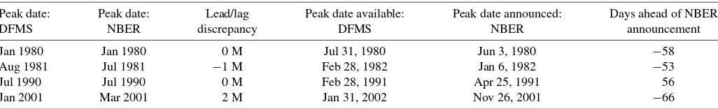
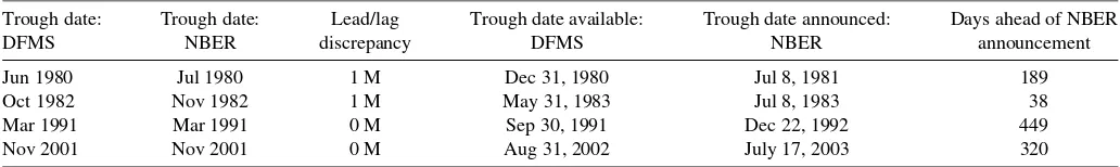
Tables 1–4 describe the real-time performance of the DFMS model and the MHP algorithm. The first column gives the turn-ing point date assigned in real time by the DFMS model or MHP algorithm. In other words, this column records the date of any new turning points established by the methods. If this turn-ing point date has a correspondturn-ing NBER turnturn-ing point, the sec-ond column gives this NBER date, and the third column records the discrepancy in months between the NBER date and the date in column 1. The fourth column gives the month in which the date in column 1 would have been available. For example, the first entry in column 4 of Table 1 is July 31, 1980. This is the first date at which the DFMS model, using the dataset available, would have revealed the January 1980 peak in column 1. The
Table 1. Business cycle peak dates obtained in real time—NBER and DFMS model
Peak date: Peak date: Lead/lag Peak date available: Peak date announced: Days ahead of NBER
DFMS NBER discrepancy DFMS NBER announcement
Jan 1980 Jan 1980 0 M Jul 31, 1980 Jun 3, 1980 −58 Aug 1981 Jul 1981 −1 M Feb 28, 1982 Jan 6, 1982 −53 Jul 1990 Jul 1990 0 M Feb 28, 1991 Apr 25, 1991 56 Jan 2001 Mar 2001 2 M Jan 31, 2002 Nov 26, 2001 −66
Table 2. Business cycle trough dates obtained in real time—NBER and DFMS model
Trough date: Trough date: Lead/lag Trough date available: Trough date announced: Days ahead of NBER
DFMS NBER discrepancy DFMS NBER announcement
Jun 1980 Jul 1980 1 M Dec 31, 1980 Jul 8, 1981 189 Oct 1982 Nov 1982 1 M May 31, 1983 Jul 8, 1983 38 Mar 1991 Mar 1991 0 M Sep 30, 1991 Dec 22, 1992 449 Nov 2001 Nov 2001 0 M Aug 31, 2002 July 17, 2003 320
fifth column gives the date the NBER announced the turning point date in column 2. The final column gives the amount of time before the NBER date that the turning point from the dat-ing methods would have been available, which is the amount of time the date in column 4 anticipates that in column 5.
We begin with Tables 1 and 2, which show the results for the DFMS model. The DFMS model identifies eight turning points in real time, each of which corresponds to a NBER turn-ing point. Thus, the DFMS model does not generate any false positives. The DFMS model also identifies these eight turning points with a high level of accuracy. In particular, for seven of the eight turning points, the turning point date identified in real time is within one month of the NBER date. For the remaining turning point, the peak of the 2001 recession, the date identified by the model is two months from the NBER date.
For business cycle peaks, the DFMS model does not show any systematic improvement over the NBER in the speed at which it identifies turning points. Indeed, the DFMS model would have identified the four peaks in the sample roughly one month after the NBER announcement on average, with a maximum lag time of two months. However, the DFMS model would have identified business cycle troughs much more quickly than the NBER. The average lead time for the four troughs in the sample is 249 days, or about 8 months, with a maximum lead time of 449 days for the 1991 business cy-cle trough. Interestingly, the increase in speed with which the DFMS algorithm identifies business cycle troughs does not come with a noticeable loss of accuracy in identifying the NBER date. Indeed, the business cycle trough dates identified in real time are all within one month of their corresponding NBER date. Given that the DFMS model treats business cycle peak and trough episodes symmetrically, its improved timeli-ness over the NBER for troughs but not peaks is suggestive of an asymmetry in the NBER approach. One explanation for this is that the NBER may have an asymmetric loss function for valuing errors made in establishing the dates of business cycle peaks versus troughs.
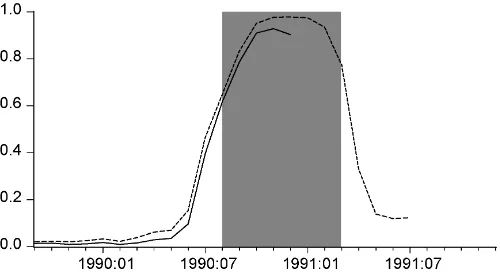
The results in Tables 1 and 2 are derived from a combination of the recession probabilities, P(St =1|T), with the dating
rule used to convert these recession probabilities into recession dates. For reference, Figures 1–4 plot the values of the real-time recession probabilities used to date each peak and trough in the sample. That is, these figures show a sequence ofP(St=1|T)
that was available at the vintage for which the business cycle peak or trough was first identified.
Tables 3 and 4 report the performance of the MHP algorithm in dating turning points in real time. Similarly to the DFMS model, the MHP algorithm also identifies eight turning points, each of which corresponds to a NBER turning point date. How-ever, these turning points are identified less accurately in gen-eral than is the case for the DFMS model. In particular, four of the turning points are at least two months from their cor-responding NBER date, with the peaks of the 1980 and 2001 recessions both six months from the NBER date.
Similarly to the DFMS model, the MHP algorithm does not show any systematic improvement over the NBER in the speed with which business cycle peaks are identified, but does show an improvement in timeliness for business cycle troughs. In particular, the MHP algorithm identified the four business cy-cle troughs in the sample an average of 166 days, or about 5.5 months, ahead of the NBER announcement. Although still a substantial increase in timeliness, it is a smaller improvement than that achieved by the DFMS model.
4.3 Revisions of Business Cycle Dates
The NBER has made revisions to previously established business cycle turning point dates, most recently in 1975. How-ever, the NBER’s Business Cycle Dating Committee has not revised any of the eight turning point dates it has established in real time since its inception in 1978. Does this rigidity suggest that the NBER’s business cycle dates are no longer consistent with the data? Or does it instead suggest that data revealed since the establishment of these turning point dates have not altered conclusions about their timing? In this section we provide some evidence on these questions.
We can evaluate the importance of data revisions for estab-lishing business cycle turning point dates by tracking revisions
Table 3. Business cycle peak dates obtained in real time—NBER and MHP algorithm
Peak date: Peak date: Lead/lag Peak date available: Peak date announced: Days ahead of NBER
MHP NBER discrepancy MHP NBER announcement
Jul 1979 Jan 1980 6 M May 31, 1980 Jun 3, 1980 3 May 1981 Jul 1981 2 M Feb 28, 1982 Jan 6, 1982 −53 Jul 1990 Jul 1990 0 M Mar 31, 1991 Apr 25, 1991 25 Sep 2000 Mar 2001 6 M Nov 30, 2001 Nov 26, 2001 −4
Chauvet and Piger: Business Cycle Dating Methods 47
Table 4. Business cycle trough dates obtained in real time—NBER and MHP algorithm
Trough date: Trough date: Lead/lag Trough date available: Trough date announced: Days ahead of NBER
MHP NBER discrepancy MHP NBER announcement
Jul 1980 Jul 1980 0 M Apr 30, 1981 Jul 8, 1981 69 Oct 1982 Nov 1982 1 M Jul 31, 1983 Jul 8, 1983 −23 Jul 1991 Mar 1991 −4 M Feb 28, 1992 Dec 22, 1992 298 Oct 2001 Nov 2001 1 M Aug 31, 2002 July 17, 2003 320
Figure 1. Real-time probabilities of recession determining the peak (—–) and trough (- - - - -) of the 1980 recession, and NBER recession (shaded).
Figure 2. Real-time probabilities of recession determining the peak (—–) and trough (- - - - -) of the 1981–1982 recession, and NBER re-cession (shaded).
Figure 3. Real-time probabilities of recession determining the peak (—–) and trough (- - - - -) of the 1990–1991 recession, and NBER re-cession (shaded).
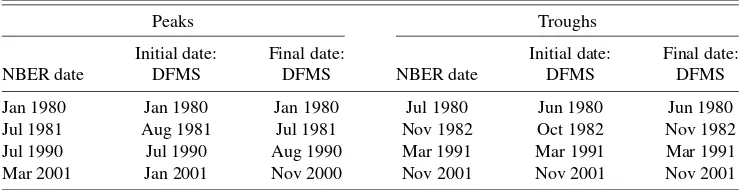
to the dates established in real time using the formal business cycle dating rules evaluated in this article. Given the superior performance of the DFMS model for mimicking the NBER dates established in real time, we focus on this approach. In particular, we apply the DFMS model to the most recent vin-tage of data available in our dataset, June 2006, and obtain a chronology of business cycle turning point dates. We then com-pare the business cycle turning point dates established in real time by the DFMS model to those established using the most recent vintage of data. Table 5 contains this comparison.
The results in Table 5 demonstrate that in most cases, data revisions do not appear to be an important factor for determin-ing the timdetermin-ing of business cycle turndetermin-ing points. In particular, for seven of the eight turning points in the sample, the date es-tablished by the DFMS model using the final vintage of data available is within one month of that established in real time. Indeed, for four of the eight turning points there is no revision to the turning point date established in real time.
The single case where the real-time business cycle date is re-vised by more than one month, namely, the peak of the 2001 recession, merits further discussion. Note that the peak of the 2001 recession is established by the DFMS model in real time to be January of 2001, two months prior to the March 2001 peak established by the NBER. From Table 1, this peak date would not have been available from the DFMS model until two months after the official announcement by the NBER. Thus, the initial date established by the DFMS model is already based on more information than was available to the NBER. Further, this peak date is moved an additional two months earlier, to Novem-ber of 2000, when the DFMS model is applied to the June 2006 vintage of data. Note that data available in June 2006 is not nec-essary for the DFMS model to make this revision. In particular,
Figure 4. Real-time probabilities of recession determining the peak (—–) and trough (- - - - -) of the 2001 recession, and NBER recession (shaded).
Table 5. Revisions to business cycle dates: DFMS model
Peaks Troughs
Initial date: Final date: Initial date: Final date: NBER date DFMS DFMS NBER date DFMS DFMS
Jan 1980 Jan 1980 Jan 1980 Jul 1980 Jun 1980 Jun 1980 Jul 1981 Aug 1981 Jul 1981 Nov 1982 Oct 1982 Nov 1982 Jul 1990 Jul 1990 Aug 1990 Mar 1991 Mar 1991 Mar 1991 Mar 2001 Jan 2001 Nov 2000 Nov 2001 Nov 2001 Nov 2001
the revision to November of 2000 would have first been avail-able from the DFMS model by the July 2002 vintage. In sum, data revealed after the official announcement by the NBER of the March 2001 peak seem to be consistent with this peak oc-curring somewhat earlier, and provide one example suggestive that an established NBER date may be inconsistent with revised data.
Although not revealed in Table 5, the trough of the 2001 re-cession is also an interesting case for investigating the effects of additional and revised data on conclusions about turning point dates. In particular, from Table 2, the DFMS model would have first established the trough date of November 2001 by the end of August of 2002. However, for a brief period for vintages in mid-2003, the recession probabilities from the DFMS model for 2002 and 2003 rose significantly to levels consistent with a continuation of the 2001 recession. This was the result of very weak employment data observed in 2002 and 2003, or the so-called “jobless recovery.” By the end of 2003, the reces-sion probabilities would have returned to levels consistent with the previously established trough date of November 2001. This episode demonstrates that the caution exercised by the NBER in establishing the trough of the 2001 recession may have been justified, particularly if their primary objective is to establish turning point dates that are unlikely to need revision.
5. CONCLUSIONS
This article investigates the ability of formal rules to establish business cycle turning point dates in real time. Both methods studied, a nonparametric algorithm given in Harding and Pagan (2003) and the dynamic-factor Markov-switching model as in Chauvet (1998), identify the NBER turning point dates in real time with reasonable accuracy, and with no instances of false positives. Both approaches also provide improvements over the NBER in the timeliness with which they identify business cy-cle troughs, but provide no such improvement for business cycle peaks. Comparing the two methods, the dynamic-factor Markov-switching model identifies NBER turning point dates more accurately, as well as identifies business cycle troughs with a larger lead.
ACKNOWLEDGMENTS
We thank Jon Faust, Robert Rasche, two anonymous refer-ees, and seminar participants at the 2005 Winter Meetings of the Econometric Society for helpful comments. Research as-sistance by Michelle Armesto and Garrett Holland was invalu-able in the completion of this project. We owe special thanks
to Robert Rasche for his assistance in obtaining the real-time dataset. We are also grateful to Don Harding for sharing his Gauss code. Much of this article was completed while Piger was a Senior Economist at the Federal Reserve Bank of St. Louis. The views expressed in this article should not be interpreted as those of the Federal Reserve Bank of St. Louis or the Federal Reserve System.
APPENDIX: SOURCES OF REAL–TIME DATA
A.1 Real Personal Income Excluding Transfer Payments
For vintages from November 1976 through March 1990, data for real personal income excluding transfer payments were collected fromBusiness Conditions Digest.For vintages from April 1990 through December 1995, data for real personal income excluding transfer payments were collected from the
Survey of Current Business. For vintages from January 1996 through June 2006, nominal personal income, nominal dis-posable personal income, and real disdis-posable personal income were collected from the Federal Reserve Bank of St. Louis AL-FRED database, whereas data for nominal transfer payments were collected fromEconomic Indicators,Business Statistics, theSurvey of Current Business, and data archives maintained by the Federal Reserve Bank of St. Louis. Data for real per-sonal income excluding transfer payments were then formed by subtracting nominal transfer payments from nominal personal income, and dividing by the ratio of nominal to real disposable personal income.
A.2 Real Manufacturing and Trade Sales
For vintages from November 1976 through March 1990, data for real manufacturing and trade sales were collected from Busi-ness Conditions Digest, whereas for vintages from April 1990 through December 1995, real manufacturing and trade sales data were collected from theSurvey of Current Business. For vintages from January 1996 through June 2006, real manufac-turing and trade sales data were collected fromBusiness Cycle Indicators,Business Statistics, theSurvey of Current Business, and data archives maintained by the Federal Reserve Bank of St. Louis.
For a small number of individual vintages, there were gaps in the data available. These missing data were filled in using the following strategy. Suppose that for the Rth vintage, we are missing data from periodt tot+k. Denote these missing data asYtR,YtR+1, . . . ,YtR+k. Suppose that data are available for
Chauvet and Piger: Business Cycle Dating Methods 49
YtR−−1h,YtR−h, . . . ,YtR+−kh,YtR+−kh+1, as well as forYtR−1andYtR+k+1. Our imputed value forYjR, denotedYˆjR, is then given by
ˆ
YjR= ˆYjR−1Y
R−h j
YjR−−1h r
1
r2
1/(k+2)
, j=t, . . . ,t+k,
wherer1=YtR+k+1/Y R
t−1,r2=Y R−h t+k+1/Y
R−h
t−1 , and the recursion
is initialized withYˆtR−1=YtR−1.
In words, this imputation formula fills in the missing data for periodjusing the actual growth rate observed in periodjfrom the data recorded at vintageR−h (the first bracketed term) modified by an amount that does not vary with j(the second bracketed term). This modification ensures that the difference in total growth observed from periodt−1 to periodt+k+1 using data from vintagesRandR−his spread evenly over the periodttot+k+1.
[Received April 2005. Revised February 2007.]
REFERENCES
Boehm, E., and Moore, G. H. (1984), “New Economic Indicators for Australia, 1949–1984,”Australian Economic Review, 68, 34–56.
Bry, G., and Boschan, C. (1971),Cyclical Analysis of Time Series: Selected Procedures and Computer Programs, New York: National Bureau of Eco-nomic Research.
Burns, A. F., and Mitchell, W. A. (1946),Measuring Business Cycles, New York: National Bureau of Economic Research.
Chauvet, M. (1998), “An Econometric Characterization of Business Cycle Dy-namics With Factor Structure and Regime Switching,”International Eco-nomic Review, 39, 969–996.
Chauvet, M., and Hamilton, J. (2006), “Dating Business Cycle Turning Points in Real Time,” inNonlinear Time Series Analysis of Business Cycles, eds. C. Milas, P. Rothman, and D. Van Dijk, Amsterdam: Elsevier Science, pp. 1–54.
Chauvet, M., and Piger, J. (2003), “Identifying Business Cycle Turning Points in Real Time,”Federal Reserve Bank of St. Louis Review, 85, 47–61. Croushore, D., and Stark, T. (2001), “A Real-Time Data Set for
Macroecono-mists,”Journal of Econometrics, 105, 111–130.
Hamilton, J. D. (1989), “A New Approach to the Economic Analysis of Non-stationary Time Series and the Business Cycle,”Econometrica, 57, 357–384. Harding, D., and Pagan, A. (2003), “A Comparison of Two Business Cycle Dat-ing Methods,”Journal of Economic Dynamics and Control, 27, 1681–1690. (2006), “Synchronization of Cycles,”Journal of Econometrics, 132, 59–79.
Kim, C.-J., and Nelson, C. R. (1998), “Business Cycle Turning Points, a New Coincident Index, and Tests of Duration Dependence Based on a Dynamic Factor Model With Regime Switching,”Review of Economics and Statistics, 80, 188–201.
Layton, A. P. (1996), “Dating and Predicting Phase Changes in the U.S. Busi-ness Cycle,”International Journal of Forecasting, 12, 417–428.
Stock, J. H., and Watson, M. W. (1989), “New Indexes of Coincident and Lead-ing Economic Indicators,”NBER Macroeconomics Annual, 4, 351–393.
(1991), “A Probability Model of the Coincident Economic Indicators,” inLeading Economic Indicators: New Approaches and Forecasting Records, eds. K. Lahiri and G. H. Moore, Cambridge, U.K.: Cambridge University Press, pp. 63–90.
Watson, M. W. (1994), “Business Cycle Durations and Postwar Stabilization of the U.S. Economy,”American Economic Review, 84, 24–46.