(ebook ) Mathematics Alder Multivariate Calculus

(1)

2C2 Multivariate Calculus

Michael D. Alder

(2)

(3)

Chapter 1 Introduction

It is the nature of things that every syllabus grows. Everyone who teaches it wants to put his favourite bits in, every client department wants their precious fragment included.

This syllabus is more stuffed than most. The recipes must be given; the reasons why they work usually cannot, because there isn’t time. I dislike this myself because I like understanding things, and usually forget recipes unless I can see why they work.

I shall try, as far as possible, to indicate by “Proofs by arm-waving” how one would go about understanding why the recipes work, and apologise in ad-vance to any of you with a taste for real mathematics for the crammed course. Real mathematicians like understanding things, pretend mathematicians like knowing tricks. Courses like this one are hard for real mathematicians, easy for bad ones who can remember any old gibberish whether it makes sense or not.

I recommend that you go to the Mathematics Computer Lab and do the following:

Under the Apple icon on the top line select Graphing Calculator and double click on it.

When it comes up, click on demos and select the full demo. Sit and watch it for a while.

When bored press the<tab>key to get the next demo. Press<shift><tab> to go backwards.

(8)

8 CHAPTER 1. INTRODUCTION

When you get to the graphing in three dimensions of functions with two variablesx and y, click on the example text and press <return/enter>. This will allow you to edit the functions so you can graph your own. Try it and see what you get for functions like

z =x2₊_y2 _{case 1}

z =x2₋_y2 _{case 2}

z =xy case 3

z = 4₋x2₋_y2 _{case 4}

z =xy₋x3₋_y2 _{+ 4} _{case 5}

If you get a question in a practice class asking you about maxima or minima or saddle points, nick off to the lab at some convenient time and draw the picture. It is worth 1000 words. At least.

I also warmly recommend you to run Mathematica or MATLAB and try the DEMO’s there. They are a lot of fun. You could learn a lot of Mathematics just by reading the documentation and playing with the examples in either program.

I don’t recommend this activity because it will make you better and purer people (though it might.) I recommend it because it is good fun and beats watching television.

(9)

Chapter 2 Optimisation

2.1 The Second Derivative Test

I shall work only with functions

f : R2 _→_R

x y

f

x y

[eg. f

x y

=z =xy₋x5_/5₋_y3_{/3 + 4 ]}

This has as its graph a surface always, see figure 2.1

Figure 2.1: Graph of a function from R2 to R

(10)

10 CHAPTER 2. OPTIMISATION

The first derivative is

which is, at a point

a b

just a pair of numbers.

[eg. f

This matrix should be thought of as a linear map from R2 toR:

[₋13,₋7]

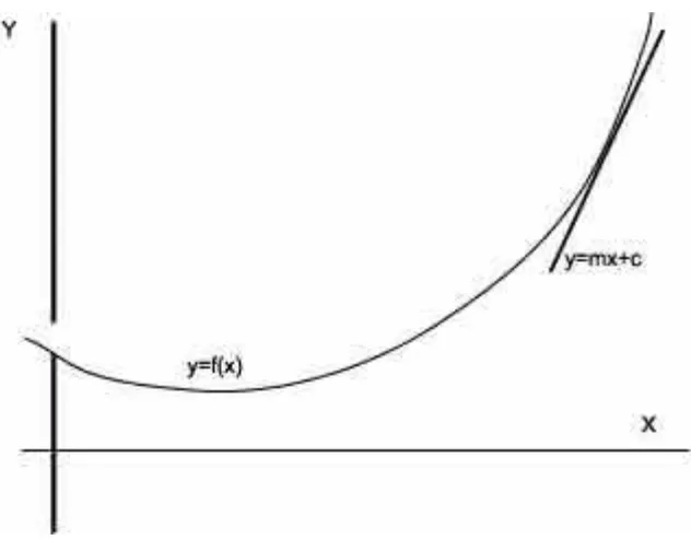
This is just the two dimensional version ofy=mx+cand has graph a plane which is tangent tof

at a point and m being the derivative at that point, as in figure 2.2.

(11)

2.1. THE SECOND DERIVATIVE TEST 11

Figure 2.2: Graph of a function from R toR

Definition 2.1. If f :R2 _→ R is differentiable and

a b

is a critical point of f then

∂f ∂x,

∂f ∂y

a b

= [0,0].

Remark 2.1.1. I deal with maps f :Rn _→R when n= 2, but generalising to larger n is quite trivial. We would have that f is differentiable at a_∈Rn if and only if there is a unique affine (linear plus a shift) map from Rn to R tangent tofata. The linear part of this then has a (row) matrix representing

it

∂f ∂x1

, ∂f ∂x2

,_{· · ·} , ∂f ∂xn

x=a

Remark 2.1.2. We would like to carry the old second derivative test through from one dimension to two (at least) to distinguish between maxima, min-ima and saddle points. This remark will make more sense if you play with the DEMO’s program on the Graphing Calculator and plot the five cases mentioned in the introduction.

I sure hope you can draw the surfacesx2₊_y2 _and_x2₋_y2_{, because if not you}

(12)

Definition 2.2. A quadratic form on R2 is a function f :R2 _→R which is a sum of termsxp_yq _where_{p, q} _∈_N_{(the natural numbers: 0,1,2,3,}_{. . .) and}

p+q _≤2 and at least one term has p+q= 2.

Definition 2.3. [alternative 1:] A quadratic form onR2 is a function f :R2 _→R

which can be written

f

for some numbers a,b,c,d,e,gand not all of a,b,c are zero.

Definition 2.4. [alternative 2:] A quadratic form onR2 is a function f :R2 _→R

which can be written

f

Remark 2.1.3. You might want to check that all these 3 definitions are equivalent. Notice that this is just a polynomial function of degree two in two variables.

Definition 2.5. Iff :R2 _→Ris twice differentiable at

the second derivative is the matrix in the quadratic form

[x₋a, y₋b]

Remark 2.1.4. When the first derivative is zero, it is the “best fitting quadratic” to f at

a b

, although we need to add in a constant to lift it up so that it is “more than tangent” to the surface which is the graph of f at

a b

(13)

Theorem 2.1. If the determinant of the second derivative is positive at

a b

for a continuously differentiable function f having first derivative zero at

a b

, then in a neighbourhood of

a b

, f has either a maximum or a

min-imum, whereas if the determinant is negative then in a neighbourhood of

a b

, f is a saddle point. If the determinant is zero, the test is

uninforma-tive.

“Proof ” by arm-waving: We have that if the first derivative is zero, the

second derivative at

a b

of f is the approximating quadratic form from

Taylor’s theorem, so we can work with this (second order) approximation to

f in order to decide what shape (approximately) the graph of f has.

The quadratic approximation is just a symmetric matrix, and all the informa-tion about the shape of the surface is contained in it. Because it is symmetric, it can be diagonalisedby an orthogonal matrix, (ie we can rotate the surface until the quadratic form matrix is just

a 0 0 b

We can now rescale the new x and y axes by dividing the x by _|a_| and the y

by _|b_|. This won’t change the shape of the surface in any essential way.

This means all quadratic forms are, up to shifting, rotating and stretching

et cetera. We do not have to actually do the diagonalisation. We simply note that the determinant in the first two cases is positive and the determinant is not changed by rotations, nor is the sign of the determinant changed by

(14)

zero and if

D2f

is continuous on a neighbourhood of

f has a local minimum at

f has a local maximum at

a b

.

“Proof ”The trace of a matrix is the sum of the diagonal terms and this is also unchanged by rotations, and the sign of it is unchanged by scalings. So again we reduce to the four possible basic quadratic forms

and the trace distinguishes betweeen the first two, being positive at a min-imum and negative at a maxmin-imum. Since the two diagonal terms have the same sign we need only look at the sign of the first.

Example 2.1.1. Find and classify all critical points of

(15)

at a critical point, this is the zero matrix [0,0] so y= 4x3 _and _y₌ 1

and there are three critical points

is a saddle point.

D2_f maximum or a minimum.

D2_f

(16)

(17)

Chapter 3 Constrained Optimisation

3.1 Lagrangian Multipliers

A function may be given not onR2 but on some curve inR2. (More generally on some hypersurface is Rn_).

Finding critical points in this case is rather different.

Example 3.1.1. Definef :R2 _→R by

x y

x2₋_y2_.

Find the maxima and minima of f on the unit circle

S1 =

x y

∈R2 :x2+y2 = 1

.

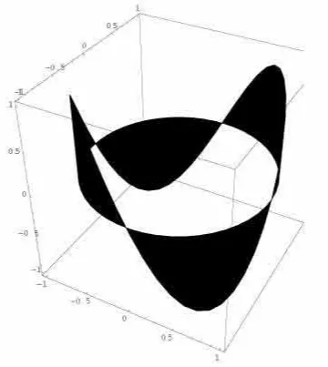
Plotting a few points we see f is zero at x = _±y, negative and a minimum at x = 0y = _±1, positive and a maximum at x = _±1y = 0. Better yet we use Mathematica and type in:

ParametricPlot3D[_{Cos[t],Sin[t],s*Sin[2t]_},_{t,0,2π_},_{s,0,1_},PlotPoints->50]

It is obvious that Df = h∂f_∂x,∂f_∂yi is zero only at the origin - which is not much help since the origin isn’t on the circle.

Q 3.1.2 How can we solve this problem? (Other than drawing the graph)

(18)

18 CHAPTER 3. CONSTRAINED OPTIMISATION

(19)

3.1. LAGRANGIAN MULTIPLIERS 19

Answer 1Express the circle parametrically by ’drawing’ the curve

eg x= cost y= sint

t_∈[0,2π)

Then f composed with the map

It is interesting to observe that the function x2₋_y2 _{restricted to the circle}

is just cos 2t.

Answer 2 (Lagrange Multipliers)

Observe that iff has a critical point on the circle, then

∇f =

which points in the direction where f is increasing most rapidly, must be normal to the circle. (Since if there was a component tangent to the circle, f couldn’t have a critical point there, it would be increasing or decreasing in their direction.)

is normal to the circle from first semester. pointing in the same direction (or maybe the exactly opposite direction), ie

(20)

are two possibilities.

If x ₆= 0 then 2x = 2λx _⇒ λ = 1 whereupon y = ₋y _⇒ y = 0 and on

are the other two.

It is easy to work out which are the maxima and which the minima by plugging in values.

Remark 3.1.1. The same idea generalises for maps

f :Rn_→R

with the problem:

Find the critical points of f subject to

(21)

We have two ways of proceeding: one is to parametise the hypersurface given by the _{gi} by finding

M :Rn−k _→Rn

such that every y _∈ Rn such that gi(y) = 0 for all i comes from some

p_∈Rn−k_{, preferably only one.}

Thenf_◦M :Rn−k_→_R _{can have its maxima and minima found as usual by}

setting

D(f _◦M) = [0,0, . . . ,0 | {z }

n−k

]

Or we can find _∇f(x) and_∇gi(x).

Then:

Proposition 3.1.1. x is a critical point of f restricted to the set

{gi(x) = 0; 1≤i≤k}

provided _∃ λ1, λ2, . . . λk ∈R

∇f(x) =

1

X

i=1,K

λi∇gi(x)

“Proof ” _∇gi(x) is normal to the ith constraint and the hypersurface is

given by k constraints which (we hope) are all independent. If you think of k tangents at the point x, you can see them as intersecting hyperplanes, the dimension of the intersection being, therefore, n₋k.

∇f cannot have a component along any of the hyperplanes at a critical point, ie_∇f(x) is in the span of thek normal vectors _∇gi(x) : 1≤i≤k.

Example 3.1.2. Find the critical points of f

x y

=x+y2 _{subject to the}

constraintx2 ₊_y2 _{= 4.}

Solution We have_∇f

x y

=

∂f ∂x ∂f ∂y

=

1 2y

and

g :R2 _→ R

x y

(22)

as the constrained set, with

∇g = so the critical points are at

If you think about f

(23)

Figure 3.3: Graph of x+y2 _{over unit circle}

So a minimum occurs at x=−2

y= 0 a local minimum at

x= 2

y= 0 and maxima at

x= 1/4 y = ±√₂15

(24)

(25)

Chapter 4 Fields and Forms

4.1 Definitions Galore

You may have noticed that I have been careful to write vectors in Rn _as

vertical columns _

   

x1

x2

... xn



   

and in particular

x y

∈R2 and not (x, y)_∈R2.

You will have been, I hope, curious to know why. The reason is that I want to distinguish between elements of two very similar vector spaces, R2 and R2∗_.

Definition 4.1. Dual Space

∀n_∈Z+,

Rn∗ ,L(Rn_,_R)

is the (real) vector space of linear maps fomRn_to_R_{, under the usual addition}

and scaling of functions.

Remark 4.1.1. You need to do some checking of axioms here, which is soothing and mostly mechanical.

Remark 4.1.2. Recall from Linear Algebra the idea of an isomorphism of vector spaces. Intuitively, if spaces are isomorphic, they are pretty much the same space, but the names have been changed to protect the guilty.

(26)

26 CHAPTER 4. FIELDS AND FORMS

Remark 4.1.3. The spaceRn∗ _{is isomorphic to}_Rn _{and hence the dimension}

of Rn∗ _is _{n. I shall show that this works for} _R2∗ _{and leave you to verify the} general result.

Proposition 4.1.1. R2∗ _{is isomorphic to}_R2

ProofFor any f _∈R2∗_{, that is any linear map from} _R2 _to_{R, put}

Then f is completely specified by these two numbers since

∀

Since f is linear this is:

xf

This gives a map

α:L(R2, R)_−→R2

wherea and b are as defined above.

This map is easily confirmed to be linear. It is also one-one and onto and has inverse the map

β :R2 _−→L(R2, R)

Consequently α is an isomorphism and the dimension of R2∗ must be the same as the dimension of R2 which is 2.

(27)

4.1. DEFINITIONS GALORE 27

I shall write [a, b]_∈R2∗ _{for the linear map}

[a, b] : R2 _−→R

x y

ax+by

Then it is natural to look for a basis forR2∗ _{and the obvious candidate is}

([1,0],[0,1])

The first of these sends x y

x

which is often called the projection on x. The other is the projection on y. It is obvious that

[a, b] =a[1,0] +b[0,1]

and so these two maps span the space L(R2_,_R_{). Since they are easily shown}

to be linearly independent they are a basis. Later on I shall use dx for the map [1,0] anddyfor the map [0,1]. The reason for this strange notation will also be explained.

Remark 4.1.5. The conclusion is that although different, the two spaces are almost the same, and we use the convention of writing the linear maps as row matrices and the vectors as column matrices to remind us that (a) they are different and (b) not very different.

Remark 4.1.6. Some modern books on calculus insist on writing (x, y)T _for

a vector inR2. T is just the matrix transpose operation. This is quite intel-ligent of them. They do it because just occasionally, distinguishing between (x, y) and (x, y)T _matters.

Definition 4.2. An element of Rn∗ is called a covector. The space Rn∗ is called the dual spaceto Rn, as was hinted at in Definition 4.1.

Remark 4.1.7. Generally, if _V is any real vector space, _V∗ _{makes sense.} If _V is finite dimensional, _V and _V∗ _{are isomorphic (and if} _V _is _not _finite dimensional,_V and_V∗ _are _NOT_{isomorphic. Which is one reason for caring} about which one we are in.)

Definition 4.3. Vector Field A vector field onRn is a map

(28)

A continuous vector field is one where the map is continuous, a differen-tiable vector field one where it is differendifferen-tiable, and a smooth vector field is one where the map is infinitely differentiable, that is, where it has partial derivatives of all orders.

Remark 4.1.8. We are being sloppy here because it is traditional. If we were going to be as lucid and clear as we ought to, we would define a space of tangents toRn at each point, and a vector field would be something more than a map which seems to be going to itself. It is important to at least grasp intuitively that the domain and range ofV are different spaces, even if they are isomorphic and given the same name. The domain of V is a space of places and the codomain of V (sometimes called the range) is a space of “arrows”.

Definition 4.4. Differential 1-Form A differential 1-form on Rn or cov-ector field onRn is a map

ω :Rn_→R∗n

It issmooth when the map is infinitely differentiable.

Remark 4.1.9. Unless otherwise stated, we assume that all vector fields and forms are infinitely differentiable.

Remark 4.1.10. We think of a vector field on R2 as a whole stack of little arrows, stuck on the space. By taking the transpose, we can think of a differential 1-form in the same way.

If V : R2 _→R2 is a vector field, we think of V

a b

as a little arrow going

from

x y

to

x+a

y+b

.

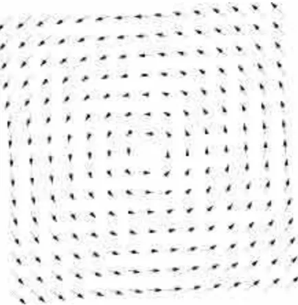
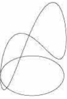
Example 4.1.1. Sketch the vector field onR2 given by

V

x y

=

−y x

Because the arrows tend to get in each others way, we often scale them down in length. This gives a better picture, figure 4.1. You might reasonably look at this and think that it looks like what you would get if you rotated R2 anticlockwise about the origin, froze it instantaneously and put the velocity vector at each point of the space. This is 100% correct.

Remark 4.1.11. We can think of a differential 1-form on R2 _{in exactly the}

(29)

Figure 4.1: The vector field [₋y, x]T

covector fields or 1-forms are not usually distinguished from vector fields as long as we stay onRn _{(which we will mostly do in this course). Actually, the}

algebra is simpler if we stick to 1-forms.

So the above is equally a handy way to think of the 1-form ω : R2 _−→R2∗

x y

(₋y, x)

Definition 4.5. i,

1 0

and j ,

0 1

when they are used in R2.

Definition 4.6. i , 

 1 0 0



 and j , 

 0 1 0



 and k , 

 0 0 1



 when they are

used in R3.

This means we can write a vector field in R2 as P(x, y)i+ Q(x, y)j

and similarly inR3:

(30)

Definition 4.7. dxdenotes the projection mapR2 _−→Rwhich sends

x y

to x. dy denotes the projection map

x y

y The same symbols dx, dy are used for the projections from R3 _{along with} _{dz. In general we have} _dxi

fromRn to R sends



   

x1

x2

... xn



   

xi

Remark 4.1.12. It now makes sense to write the above vector field as

−y i +x j

or the corresponding differential 1-form as

−y dx+ x dy

This is more or less the classical notation.

Why do we bother with having two things that are barely distinguishable? It is clear that if we have a physical entity such as a force field, we could cheerfully use either a vector field or a differential 1-form to represent it. One part of the answer is given next:

Definition 4.8. A smooth 0-form on Rn is any infinitely differentiable map (function)

f :Rn _→R.

Remark 4.1.13. This is, of course, just jargon, but it is convenient. The reason is that we are used to differentiating f and if we do we get

Df : Rn _−→L(Rn_,_R)

x Df(x) =

∂f ∂x1

, ∂f ∂x2

, . . . ∂f ∂xn

(x)

This I shall write as

(31)

and, lo and behold, when f is a 0-form on Rn df is a differential 1-form on Rn. When n = 2 we can takef :R2 _−→R as the 0-form and write

df = ∂f

∂x dx + ∂f ∂y dy

which was something the classical mathematicians felt happy about, the dx and the dy being “infinitesimal quantities”. Some modern mathematicians feel that this is immoral, but it can be made intellectually respectable.

Remark 4.1.14. The old-timers used to write, and come to think of it still do,

∇f(x), 

 

∂f ∂x1 ...

∂f ∂xn



 

and call the resulting vector field the gradient field of f.

This is just the transpose of the derivative of the 0-form of course.

Remark 4.1.15. For much of what goes on here we can use either notation, and it won’t matter whether we use vector fields or 1-forms. There will be a few places where life is much easier with 1-forms. In particular we shall repeat the differentiating process to get 2-forms, 3-forms and so on.

Anyway, if you think of 1-forms as just vector fields, certainly as far as visualising them is concerned, no harm will come.

Remark 4.1.16. A question which might cross your mind is, are all 1-forms obtained by differentiating 0-forms, or in other words, are all vector fields gradient fields? Obviously it would be nice if they were, but they are not. In particular,

V

x y

,

−y x

is not the gradient field _∇f for any f at all. If you ran around the origin in a circle in this vector field, you would have the force against you all the way. If I ran out of my front door, along Broadway, left up Elizabeth Street, and kept going, the force field of gravity is the vector field I am working with. Or against. The force is the negative of the gradient of the hill I am running up. You would not however, believe that, after completing a circuit and arriving home out of breath, I had been running uphill all the way. Although it might feel like it.

(32)

Definition 4.10. A 1-form which is the derivative of a 0-form is said to be

exact.

Remark 4.1.17. Two bits of jargon for what is almost the same thing is a pain and I apologise for it. Unfortunately, if you read modern books on, say theoretical physics, they use the terminology of exact 1-forms, while the old fashioned books talk about conservative vector fields, and there is no solution except to know both lots of jargon. Technically theyare different, but they are often confused.

Definition 4.11. Any 1-form on R2 will be written ω,P (x, y)dx+Q(x, y)dy.

The functionsP(x, y), Q(x, y) will be smooth whenω is, since this is what it means forω to be smooth. So they will have partial derivatives of all orders.

4.2 Integrating 1-forms (vector fields) over

curves.

Definition 4.12. I =_{x_∈R: 0_≤x_≤1_}

Definition 4.13. A smooth curve inRn is the image of a map c:I _−→Rn

that is infinitely differentiable everywhere.

It is piecewise smooth if it is continuous and fails to be smooth at only a finite set of points.

Definition 4.14. A smooth curve isoriented by giving the direction in which t is increasing fort _∈I _⊂R

Remark 4.2.1. If you decided to use some interval other than the unit interval, I, it would not make a whole lot of difference, so feel free to use, for example, the interval of points between 0 and 2π if you wish. After all, I can always mapI into your interval if I feel obsessive about it.

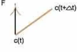
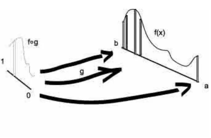
Remark 4.2.2. [Motivation] Suppose the wind is blowing in a rather er-ratic manner, over the great gromboolian plain (R2_{). In figure 4.2 you can}

(33)

4.2. INTEGRATING 1-FORMS (VECTOR FIELDS) OVER CURVES. 33

Figure 4.2: Bicycling over the Great Gromboolian Plain

Figure 4.3: An infinitesimal part of the ride

We represent the wind as a vector fieldF :R2 _−→R2. I cycle along a curved path, and at time 0 I start out at c(0) and at time t I am at c(t). I stop at time t= 1.

I am interested in the effect of the wind on me as I cycle. Att = 0 the wind is pushing me along and helping me. Att= 1 it is against me. In between it is partly with me, partly at right angles to me and sometimes partly against me.

I am not interested in what the wind is doing anywhere else.

I suppose that if the wind is at right angles to my path it has no effect (although it might blow me off the bike in real life).

The question is, how much net help or hindrance is the wind on my journey? I solve this by chopping my path up into little bits which are (almost) straight line segments.

F is the wind at where I am timet.

(34)

that this could be defined without reference to a parametrisation. The component in my direction, muliplied by the length of the path is

F _◦c(t) qc′(t) for time△t

(approximately.) qdenotes the inner or dot product.

(The component in my direction is the projection on my direction, which is the inner product of the Force with the unit vector in my direction. Usingc′ includes the “speed” and hence gives me the distance covered as a term.) I add up all these values to get the net ‘assist’ given byF.

Taking limits, the net assist is Z t=1

t=0

F(c(t)) qc′(t)dt

Example 4.2.1. The vector fieldF is given by

F

(I am in a hurricane or cyclone)

I choose to cycle in the unit (quarter) circle from

Differentiating cwe get:

c′_{(t) =}

(35)

4.2. INTEGRATING 1-FORMS (VECTOR FIELDS) OVER CURVES. 35

This is positive which is sensible since the wind is pushing me all the way. Now I consider a different path from

along the X axis to the origin, then to proceed along theY-axis finishing at

0 1

. I am going to do this path in two separate stages and then add up the answers. This has to give the right answer from the definition of what a path integral is. So my first stage has

c(t),

(which means that I am travelling at uniform speed in the negative x direc-tion.)

The ‘assist’ for this stage is Z 1

which is zero. This is not to surprising if we look at the path and the vector field.

The next stage has a new c(t):

c(t),

0 t

which goes from the origin up a distance of one unit. Z 1

This makes sense because the wind is always orthogonal to my path and has no net effect.

(36)

Remark 4.2.3. The only difficulty in doing these sums is that I might de-scribe the path and fail to give it parametrically - this can be your job. Oh, and the integrals could be truly awful. But that’s why Mathematica was invented.

4.3 Independence of Parametrisation

Suppose the path is the quarter circle from [1,0]T _{to [0,}_1]T_{, the circle being}

centred on the origin. One student might write

c: [0,1]_−→R2

c(t),

cos(π₂t) sin(π

2t)

Another might take

c: [0, π/2]_−→R2

c(t),

cos(t) sin(t)

Would these two different parametrisations of the same path give the same answer? It is easy to see that they would get the same answer. (Check if you doubt this!) They really ought to, since the original definition of the path integral was by chopping the path up into little bits and approximating each by a line segment. We used an actual parametrisation only to make it easier to evaluate it.

Remark 4.3.1. For any continuous vector field F on Rn and any differen-tiable curve c, the value of the integral of F over c does not depend on the choice of parametrisation of c. I shall prove this soon.

Example 4.3.1. For the vector fieldFon R2 _{given by}

F

x y

,

−y x

evaluate the integral of Falong the straight line joining

1 0

to

0 1

(37)

4.3. INDEPENDENCE OF PARAMETRISATION 37

Then the integral is

Rt=1

This looks reasonable enough.

Parametisation 2

Now next move along the same curve but at a different speed:

c(t),

So the integral is

(38)

So we got the same result although we moved along the line segment at a different speed. (starting off quite fast and slowing down to zero speed on arrival)

Does it always happen? Why does it happen? You need to think about this until it joins the collection of things that are obvious.

In the next proposition, [a, b],{x_∈R:a _≤x_≤b_}

Proposition 4.3.1. Ifc: [u, v]_→Rn is differentiable and ϕ: [a, b]_→ [u, v] is a differentiable monotone function with ϕ(a) = u and ϕ(b) = v and e : [a, b]_→Rn is defined bye,c_◦ϕ, then for any continuous vector field V on Rn,

Z v

u

V(c(t)) qc′(t)dt =

Z b

a

V(e(t)) qe′(t)dt.

ProofBy the change of variable formula Z

V(c(t)) qc′(t)dt =

Z

V(c(ϕ(t)) qc′(ϕ(t))ϕ′t)dt

= V(e(t)) qe′(t)dt(chain rule)

Remark 4.3.2. You should be able to see that this covers the case of the two different parametrisations of the line segment and extends to any likely choice of parametrisations you might think of. So if half the class thinks of one parametrisation of a curve and the other half thinks of a different one, you will still all get the same result for the path integral provided they do

trace the same path.

Remark 4.3.3. Conversely, if you go by different paths between the same end points you will generally get a different answer.

Remark 4.3.4. Awful Warning The parametrisation doesn’t matter but the orientation does. If you go backwards, you get the negative of the result you get going forwards. After all, you can get the reverse path for any parametrisation by just swapping the limits of the integral. And you know what that does.

Example 4.3.2. You travel from

1 0

to

−1 0

in the vector field

V

x y

,

−y x

(39)

4.4. CONSERVATIVE FIELDS/EXACT FORMS 39

1. by going around the semi circle (positive half)

2. by going in a straight line

3. by going around the semi circle (negative half)

It is obvious that the answer to these three cases are different. (b) obviously gives zero, (a) gives a positive answer and (c) the negative of it.

(I don’t need to do any sums but I suggest you do.) (It’s very easy!)

4.4 Conservative Fields/Exact Forms

Theorem 4.4.1. If V is a conservative vector field on Rn, ie V =_∇ϕ for ϕ:Rn _→Rdifferentiable, and if c: [a, b]_→R is any smooth curve, then

Z

c

V =

Z b

a

V(c(t)) qc′(t)dt

= ϕ(c(b))₋ϕ(c(a))

Proof

Z

c

V =

Z b

r=a

V(c(t)) qc′(t)dt

write

c(t) = 

   

x1(t)

x2(t)

... xn(t)



   

(40)

40 CHAPTER 4. FIELDS AND FORMS In other words, it’s the chain rule.

Corollary 4.4.1.1. For a conservative vector field, V, the integral over a curve c R_cV depends only on the end points of the curve and not on the

path.

Remark 4.4.1. It is possible to ask an innocent young student to tackle a thoroughly appalling path integral question, which the student struggles for days with. If the result in fact doesn’t depend on the path, there could be an easier way.

Example 4.4.1.

that follows the curve shown in fig-ure 4.4, a quarter of a circle with centre at [1,1]T_.

FindR_cV

(41)

4.4. CONSERVATIVE FIELDS/EXACT FORMS 41

Figure 4.4: quarter-circular path

The lazy but thoughtful student notes that V = _∇ϕ for ϕ = sin(x2 ₊_y2₎

and writes down ϕ

0 1

−ϕ

1 0

= 0 since 12 _{+ 0}2 _{= 0}2 _{+ 1}2 _{= 1.}

Which saves a lot of ink.

Remark 4.4.2. It is obviously a good idea to be able to tell if a vector field is convervative:

Remark 4.4.3. If V=_∇f for f :Rn _−→Rwe have

V

x y

,P

x y

dx+Q

x y

dy

is the corresponding 1-form where

P = ∂f

∂x Q= ∂f ∂y.

In which case

∂P ∂y =

∂2_f

∂y∂x = ∂2_f

∂x∂y = ∂Q

∂x

Soif

∂P ∂y =

∂Q ∂x then there is hope.

Definition 4.15. A 1-form on R2 is said to be closed iff ∂P

∂y − ∂Q

(42)

Remark 4.4.4. Then the above argument shows that every exact 1-form is closed. We want the converse, but at least it is easy to check if there is hope.

Example 4.4.2.

V

x y

=

2xcos(x2₊_y2₎

2ycos(x2 ₊_y2₎

has

P = 2xcos(x2+y2), Q= 2ycos(x2+y2) and

∂P

∂y = (−4xysin(x

2₊_y2_{)) =} ∂Q

∂x

So there is hope, and indeed the field is conservative: integrateP with respect tox to get, say,f and check that

∂f ∂y =Q

Example 4.4.3. NOT!

ω =₋ydx+xdy has

∂P ∂y =−1 but

∂Q ∂x = +1

So there is no hope that the field is conservative, something our physical intuitions should have told us.

4.5 Closed Loops and Conservatism

Definition 4.16. c : I _−→ Rn, a (piecewise) differentiable and continuous function is called a loop iff

c(0) =c(1)

Remark 4.5.1. IfV :Rn_→_Rn _{is conservative and} _c _{is any loop in}_Rn_,

Z

c

V= 0

(43)

4.5. CLOSED LOOPS AND CONSERVATISM 43

Proposition 4.5.1. If V is a continuous vector field on Rn and for every

loopℓ inRn,

Z

ℓ

V= 0

Then for every path c, R_cV depends only on the endpoints ofc and is inde-pendent of the path.

Proof: If there were two paths,c1 and c2 between the same end points and

Z

woud be nonzero, contradiction.

Remark 4.5.2. This uses the fact that the path integral along any path in one direction is the negative of the reversed path. This is easy to prove. Try it. (Change of variable formula again)

Proposition 4.5.2. If V : Rn _→ Rn is continuous on a connected open

set_{D ⊆} Rn

Andif R_cV is independent of the path Then V is conservative on _D

Proof: Let 0 be any point. I shall keep it fixed in what follows and define

ϕ(0)_,0

some ball centred on P, comes in to P changing only xi_{, the} _ith _component.

In the diagram in R2, figure 4.5, I come in along the x-axis.

for some positive real numbera, and the

(44)

Figure 4.5: Sneaking Home Along the X axis

We have V

for each Vi a continuous function

Rn toR, and

Where I have specified the endpoints only since V has the independence of path properly.

For every point P _{∈ D} I define ϕ( P) to be R0P V, and I can rewrite the

above equation as

(45)

Since the integration is just along the x1 line we can write

ϕ(P) =ϕ(P′_{) +}

Differentiating with respect tox1

∂ϕ

Recall the Fundamental theorem of calculus here:

to conclude that

∂ϕ

(46)

Figure 4.6: A Hole and a non-hole

Remark 4.5.4. So far I have cheerfully assumed that

V:Rn_→Rn

is a continuous vector field and

c:I _→Rn

is a piecewise differentiable curve.

There was one place where I was sneaky and definedV onR2 by

V

x y

, −1 (x2₊_y2₎3/2

x y

This is not defined at the origin. Lots of vector fields in Physics are like this. You might think that one point missing is of no consequence. Wrong! One of the problems is that we can have the integral along a loop is zero provided the loop does not circle the origin, but loops around the origin have non-zero integrals.

For this reason we often want to restrict the vector field to be continuous (and defined) over some region which has no holes in it.

It is intuitively easy enough to see what this means:

in figure 4.6, the left region has a big hole in it, the right hand one does not. Saying this is algebra is a little bit trickier.

Definition 4.17. For any sets X, Y, f :X _→Y is 1-1.

(47)

Definition 4.18. For any subset U _⊆ Rn, ∂U is the boundary of U and is defined to be the subset of Rn of points p having the property that every open ball containing p contains points ofU and points not inU.

Definition 4.19. The unit square is

x y

∈R2 : 0_≤x_≤1,0_≤y_≤1

Remark 4.5.5. ∂I2 _{is the four edges of the square. It is easy to prove that}

there is a 1-1 continuous map from ∂I2 _to _S1_{, the unit circle, which has a}

continuous inverse.

Exercise 4.5.1. Prove the above claim

Definition 4.20. _Dissimply connected iff every continuous mapf :∂I2 _−→ D extends to a continuous 1-1 map ˜f :I2 _{−→ D}_{, i.e. ˜}_f_|_∂I2 ₌_f

Remark 4.5.6. You should be able to see that it looks very unlikely that if we have a hole in _D and the map from ∂ to _D circles the hole, that we could have a continuous extension to I2. This sort of thing requires proof but is too hard for this course. It is usually done by algebraic topology in the Honours year.

Proposition 4.5.3. If F= Pi+Qj is a vector field on _{D ∈} R2 and _D is open, connected and simply connected, then if

∂Q ∂x −

∂P ∂y = 0

on_D, there is a “potential function”f :_{D −→}Rsuch that F=_∇f, that is,

Fis conservative.

(48)

(49)

Chapter 5 Green’s Theorem

5.1 Motivation

5.1.1 Functions as transformations

I shall discuss maps f :I _−→R2 and describe a geometric way of visualising them, much used by topologists, which involves thinking about I = _{x _∈ R : 0_≤ x _≤1_} as if it were a piece of chewing gum1_{. We can use the same}

way of thinking about functions f : R _−→ R. You are used to thinking of such functions geometrically by visualising the graph, which is another way of getting an intuitive grip on functions. Thinking of stretching and deforming the domain and putting it in the codomain has the advantage that it generalises to maps from R to Rn, from R2 to Rn and from R3 to Rn _for _n _{= 1,}_{2 or 3. It is just a way of visualising what is going on, and}

although Topologists do this, they don’t usually talk about it. So I may be breaking the Topologist’s code of silence here.

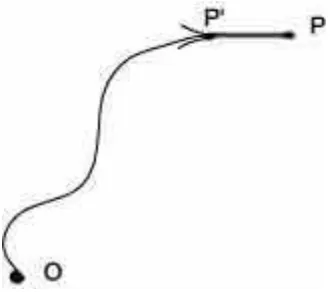
Example 5.1.1. f(x) , 2x can be thought of as taking the real line, re-garded as a ruler made of chewing gum and stretching it uniformly and moving it across to a second ruler made of, let’s say, wood. See figure 5.1 for a rather bad drawing of this.

Example 5.1.2. f(x),−x just turns the chewing gum ruler upside down and doesn’t stretch it (in the conventional sense) at all. The stretch factor

1

If, like the government of Singapore. you don’t like chewing gum, substitute putty or plasticene. It just needs to be something that can be stretched and won’t spring back when you let go

(50)

50 CHAPTER 5. GREEN’S THEOREM

Figure 5.1: The functionf(x),2x thought of as a stretching.

is₋1.

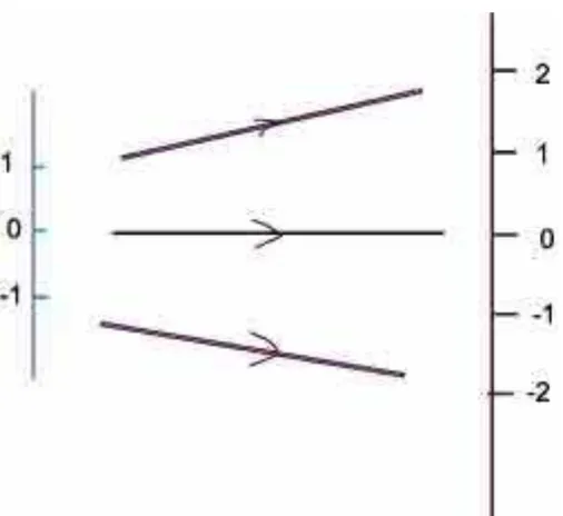
Example 5.1.3. f(x),x+ 1 just shifts the chewing gum ruler up one unit and again doesn’t do any stretching, or alternatively the stretch factor is 1. Draw your own pictures.

Example 5.1.4. f(x) , |x_| folds the chewing gume ruler about the origin so that the negative half fits over the positive half; the stretch factor is 1 when x > 0 and ₋1 when x < 0 See figure 5.2 for a picture of this map in chewing gum language.

Example 5.1.5. f(x) , x2 _{This function is more interesting because the}

amount of stretch is not uniform. Near zero it is a compression: the interval between 0 and 0.5 gets sent to the interval from 0 to 0.25 so the stretch is one half over this interval. Whereas the interval between 1 and 2 is sent to the interval between 1 and 4, so the stretch factor over the interval is three. I won’t try to draw it, but it is not hard.

Remark 5.1.1. Now I want to show you, with a particular example, how quite a lot of mathematical ideas are generated. It is reasonable to say of the functionf(x),x2 _{that the amount of stretch depends on where you are. So}

(51)

5.1. MOTIVATION 51

Figure 5.2: The functionf(x),|x_| in transformation terms.

It is plausible that this is a meaningful idea, and I can say it in English easily enough. A mathematician is someone who believes that it has to be said in Algebra before it really makes sense.

How then can we say it in algebra? We can agree that it is easy to define the stretch factor for an interval, just divide the length after by the length before, and take account of whether it has been turned upside down by putting in a minus sign if necessary. To define it at a point, I just need to take the stretch factor for small intervals around the point and take the limit as the intervals get smaller.

Saying this in algebra:

S(f, a), lim

∆→0

f(a+ ∆)₋f(a) ∆

Remark 5.1.2. This looks like a sensible definition. It may look familiar.

Remark 5.1.3. Suppose I have two maps done one after the other: R_−→g R_−→f R

If S(g, a) = 2 and S(f, g(a)) = 3 then it is obvious that S(f _◦g, a) = 6. In general it is obvious that

(52)

Figure 5.3: The change of variable formula.

Note that this takes account of the sign without our having to bother about it explicitly.

Remark 5.1.4. You may recognise this as the chain rule and S(f, a) as being the derivative of f at a. So you now have another way of thinking about derivatives. The more ways you have of thinking about something the better: some problems are very easy if you think about them the right way, the hard part is finding it.

5.1.2 Change of Variables in Integration

Remark 5.1.5. This way of thinking makes sense of the change of variables formula in integration, something which you may have merely memorised. Suppose we have the problem of integrating some function f : U _−→ R where U is an interval. I shall write [a, b] for the interval_{x_∈R:a_≤x_≤b_} So the problem is to calculate

Z b

a

f(x) dx

(53)

5.1. MOTIVATION 53

The integral is defined to be the limit of the sum of the areas of little boxes sitting on the segment [a, b]. I have shown some of the boxes. We can pull back the function f (expressed via its graph) to f _◦ g which is in a sense the “same” function– well, it has got itself compressed, in general by different amounts at different places, because g stretches I to the (longer in the picture) interval [a, b].

Now the integral off_◦g overI is obviously related to the integral of f over [a, b]. If we have a little box at t _∈I, the height of the function f_◦g at t is exactly the same as the height of f over g(t). But if the width of the box at t is ∆t, it gets stretched by an amount which is approximately g′_{(t) in going} to [a, b]. So the area of the box ong(t), which is whatg does to the box at t, is approximately the area of the box at t multiplied by g′_{(t). And since this} holds for all the little boxes no matter how small, and the approximation gets better as the boxes get thinner, we deduce that it holds for the integral:

Z 1

0

f_◦g(t)g′(t)dt = Z b

a

f(x) dx

This is the change of variable formula. It actually works even when g is not 1-1, since if g retraces its path and then goes forward again, the backward bit is negative and cancels out the first forward bit. Of course, g has to be differentiable or the formula makes no sense.2

When you do the integral

Z π/2

0

sin(t) cos(t) dt

by substituting x= sin(t), dx= cos(t) dt to get Z 1

0

x dx

you are doing exactly this “stretch factor” trick. In this caseg is the function that takes t tox = sin(t); it takes the interval from 0 to π/2 to the interval I (thus compressing it) and the function y = x pulls back to the function y = sin(t) over [0, π/2]. The stretching factor is dx= cos(t) dt and is taken care of by the differentials. We shall see an awful lot of this later on in the course.

2

(54)

Figure 5.4: A vector field or 1-form with positive “twist”.

5.1.3 Spin Fields

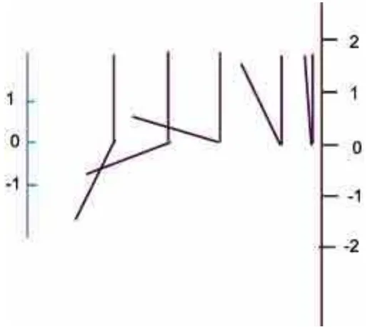
Remark 5.1.6. I hope that you can see that thinking about functions as stretching intervals and having an amount of stretch at a point is useful: it helps us understand otherwise magical formulae. Now I am ready to use the kind of thinking that we went through in defining the amount of stretch of a function at a point. Instead, I shall be looking at differential 1-forms orR2 and looking at the amount of “twist” the 1-form may have at a point of R2. The 1-form ₋ydx+xdy clearly has some, see figure 5.4

Remark 5.1.7. Think about a vector field or differential 1-form onR2 _and

imagine it is the velocity field of a moving fluid. Now stick a tiny paddle wheel in at a point so as to measure the “rotation” or “twist” or “spin” at a point.

This idea, like the amount of stretch of a function f :R_−→R is vague, but we can try to make it precise by saying it in algebra.

Remark 5.1.8. If V

x y

,P(x, y) dx+Q(x, y)dy

is the 1-form, look first atQ(x, y) along the horizontal line through the point

a b

(55)

5.1. MOTIVATION 55

Figure 5.5: The amount of rotation of a vector field

Figure 5.6: ∆Q_≈ ∂Q_∂x ∆x

If_△x is small, the Q component to the right of

a b

is

Q

a b

+∂Q

∂x△x and to the left is

Q

a b

−∂Q_∂x△x

and the spin per unit length about

a b

in the positive direction is

∂Q ∂x

Similarly there is a tendency to twist in the opposite direction given by ∂P

(56)

Figure 5.7: Path integral around a small square

So the total spin can be defined as ∂Q

∂x − ∂P

∂y

This is a function fromR2 to R.

Example 5.1.6.

ω , x2y dx+ 3y2x dy spin(ω) = 3y2₋2xy

Example 5.1.7.

ω , −y dx+x dy spin(ω) = 2

Where 2 is the constant function.

Remark 5.1.9. Another way of making the idea of ‘twist’ at a point precise would be to take the integral around a little square centred on the point and divide by the area of the square.

If the square, figure 5.7 has side 2_△ we go around each side.

From

a+_△ b_{− △}

to

a+_△ b+_△

(57)

5.2. GREEN’S THEOREM (CLASSICAL VERSION) 57

and so the path integral for this side is approximately

The side from

is affected only by theP component and the path integral for this part is approximately

with the minus sign because it is going in the negative direction. Adding up the contribution from the other two sides we get

5.2 Green’s Theorem (Classical Version)

Theorem 5.2.1. Green’s Theorem LetU _⊂R2 be connected and simply connected (has no holes in it), and has boundary a simple closed curve, that is a loop which does not intersect itself, sayℓ.

LetV be a smooth vector field

V

(58)

Figure 5.8: Adding paths around four sub-squares

Then _Z

ℓ

V=

ZZ

U

∂Q

∂x − ∂P

∂y

where the loopℓ is traversed in the positive (anticlockwise) sense.

“Proof ”I shall prove it for the particular case whereU is a square, figure 5.8. IfABCD is a square, Q is the midpoint ofAB, M of BC, N of CD, and P of DA, and if E is the centre of the square, then

Z

ABCD

V=

Z

AQEP

V+

Z

QBM E

V+

Z

M CN E

V+

Z

N DP E

V

This is trivial, since we get the integral around each subsquare by adding up the integral around each edge; the inner lines are traversed twice in opposite directions and so cancel out.

We can continue subdividing the squares as finely as we like, and the sum of the path integral around all the little squares is still going to be the path integral around the big one.

But the path integral around a very small square can be approximated by

∂Q ∂x −

∂P ∂y

(59)

5.2. GREEN’S THEOREM (CLASSICAL VERSION) 59

evaluated at the centre of the square and multiplied by its area, as we saw in the last section. And the limit of this sum is precisely the definition of the Riemann integral of

∂Q ∂x −

∂P ∂y

over the region enclosed by the square.

Remark 5.2.1. To do it for more general regions we might hope the bound-ary is reasonable and fill it with squares. This is not terribly convincing, but we can reason that other regions also have path integral over the boundary approximated by

∂Q

∂x − ∂P

∂y

×(area enclosed by shape)

Remark 5.2.2. The result for a larger collection of shapes will be proved later.

Exercise 5.2.1. Try to prove it for a triangular region, say a right-angled triangle, by chopping the triangle up into smaller triangles.

Example 5.2.1. of Green’s Theorem in use: Evaluate R_c sin(x3_)dx₊

xy+ 6dywherecis the triangular path starting at i, going by a straight line toj, then down to the origin, then back toi.

Solution: It is not too hard to do this the long way, but Green’s Theorem tells us that the result is the same as

Z Z

U

∂Q

∂x − ∂P

∂y

dx dy

whereU is the inside of the triangle, P(x, y) = sin(x3_{) and} _{Q(x, y) =}_xy_{+ 6}

This gives

Z 1

0

Z 1−x

0

(y₋0)dy dx

which I leave you to verify is 1/6.

Remark 5.2.3. While we are talking about integrals around simple loops, there is some old fashioned notation for such integrals, they often used to

write _I

c

f(t)dt

(60)

The only known use for these signs is to impress first year students with how clever you are, and it doesn’t work too well.

Example 5.2.2. Find: I

S1

(log_e(x6+ 152) + 17y) dx+ (p1 +y58₊_x) _dy

You must admit this looks horrible regarded as a path integral. It is easily seen however to be _Z

D2

(1₋17)

this is ₋16 times the area of the unit disc which is of course π So we get

−16π

Remark 5.2.4. So Green’s Theorem can be used to scare the pants off people who have just learnt to do line integrals. This is obviously extremely useful.

5.3 Spin fields and Differential 2-forms

The idea of a vector field having an amount of twist or spin at each point turned out to make sense. Now I want to consider something a bit wilder. Suppose I have a physical system which has, for each point in the plane, an amount of twist or spin associated with it. We do not need to assume this comes from a vector field, although it might. I could call such a thing a ‘twist field’ or ‘spin field’ on R2. If I did I would be the only person doing so, but there is a proper name for the idea, it is called3 _a_{differential 2-form}_.

To signal the fact that there is a number associated with each point of the plane and it matters which orientation the plane has, we write

R(x, y) dx_∧dy

for this ‘spin field’. The dx_∧dy tells us the positive direction, from x toy. If we reverse the order we reverse the sign:

dx_∧dy=₋dy_∧dx

3

(61)

5.3. SPIN FIELDS AND DIFFERENTIAL 2-FORMS 61

Remark 5.3.1. The idea makes sense, and we now have a spin field and we can ask, does it come from a vector field? Or more simply, we have a differential 2-form and we would like to know if it comes from a differential 1-form.

Given R(x, y) dx_∧dy, is there always a P dx+Q dy that gives

R(x, y) = ∂Q ∂x −

∂P ∂y ?

It is easy to see that there are lots of them.

Example 5.3.1. Let

ψ =xysin(y) dx_∧dy

be a “spin field” on R2. Is it derived from some 1-formω =P dx+Q dy?

Solution: Yes, put P = 0 and Q=x2_y_{sin(y)/2 Then}

∂Q ∂x −

∂P

∂y =xysin(y)

All I did was to set P to zero and integrate Q with respect to x. This is a bit too easy to be interesting. It stops being so silly if we do it on R3, as we shall see later.

Remark 5.3.2.It should be obvious that just as we had the derivative taking 0-forms to 1-forms, so we have a process for getting 2-forms from 1-forms. The process is called theexterior derivative, writtendand onR2 is is defined by:

Definition 5.1. Ifω,P dx+Q dyis a 1-form onR2 the exterior derivative of ω,dω, is defined by

dω ,

∂Q ∂x −

∂P ∂y

dx_∧dy

Remark 5.3.3. Although I have been doing all this on R2, it all goes over to R3 _{and indeed} _Rn _{for any larger} _{n. It is particularly important in} _R3_{, so}

I shall go through this case separately.

Remark 5.3.4. If you can believe in a ‘spin field’ in R2 you can probably believe in one onR3. Again, you can see that a little paddle wheel in a vector field flow on R3 _{could turn around as a result of different amounts of push}

(62)

any plane through the point, and the amount of twist would depend on the point and the plane chosen. If you think of time as a fourth dimension, you can see that it makes just as much sense to have a spin field onR4. In both cases, there is a point and a preferred plane and there has to be a number associated with the point and the plane. After all, twists occur in planes. This is exactly why 2-forms were invented. Another thing about them: if you kept the point fixed and varied the plane continuously until you had the same plane, only upside down, you would get the negative of the answer you got with the plane the other way up. In R3 the paddle wheel stick would be pointing in the opposite direction.

We can in fact specify the amount of spin in three separate planes, thex₋y plane, thex₋z plane, and the y₋z plane, and this is enough to be able to calculate it for any plane. This looks as though we are really doing Linear Algebra, and indeed we are.

Definition 5.2. 2-forms on R3 A smooth differential 2-form onR3 is writ-ten

ψ ,E(x, y, z) dx_∧dy+F(x, y, z) dx_∧dz+G(x, y, z) dy_∧dz where the functionsE, F, G are all smooth.

Remark 5.3.5. If you think of this as a spin field on R3 with E(x, y, z) giving the amount of twist in the x₋y plane, and similarly for F, G, you won’t go wrong. This is a useful way to visualise a differential 2-form onR3.

Remark 5.3.6. It might occur to you that I have told you how we write a differential 2-form, and I have indicated that it can be used for talking about spin fields, and told you how to visualise the spin fields and hence differential 2-forms. What I have not done is to give a formal definition of what oneis. Patience, I’m coming to this.

Example 5.3.2. Suppose the plane x+y+z = 0 in R3 is being rotated in

the positive direction when viewed from the point 

 1 1 1



, at a constant rate

of one unit. Express the rotation in terms of its projection on thex₋y,x₋z and y₋z planes.

(63)

Take a basis for the plane consisting of two orthogonal vectors in the plane of length one. There are an infinite number of choices: I pick

u=

(I got these by noticing that 

cross product with the normal to the plane to get 

finally I scaled them to have length one.) Now I write

du= √dx

which I got by telling myself that the projection onto the basis vectorushould be called du, and that it would in fact send [x, y, z]T _{to 1/}√₂ _i₋_1/√₂ _k

which is the mixture

dx And similarly for the expression for dv. Last, I write the spin as

(64)

This shows equal amounts of spin on each plane, and a negative twist on the x₋z plane, which is right. (Think about it!)

Note that the sum of the squares of the coefficients is 1. This is the amount of spin we started with. Note also that the sums are easy although they introduce the _∧ as if it is a sort of multiplication. I shall not try to justify this here. At this point I shall feel happy if you are in good shape to do the sums we have coming up.

Remark 5.3.7. It would actually make good sense to write it out using dz_∧dx instead of dx_∧dz Then the plane x+y+z = 0 with the positive orientation can be written as

1

In this form it is rather strikingly similar to the unit normal vector to the plane. Puttingdx_∧dy=kand so on, is rather tempting. It is a temptation to which physicists have succumbed rather often.

Example 5.3.3. The spin field 2 dx_∧dy+ 3dz _∧dx+ 4 dy_∧dz on R3 _is

examined by inserting a probe at the origin so that the oriented plane is again x+y+z = 0 with positive orientation seen from the point i+j+k. What is the amount of spin in this plane?

Solution 1Project the vector 2 dx_∧dy+ 3dz_∧dx+ 4 dy_∧dz on the vector

Solution 2(Physicist’s solution) Write the spin as a vector 4i+ 3j+ 2kand the normal to the oriented plane as

1

Now take the dot product to get the length of the spin (pseudo)vector: 9/√3 = 3√3. The whole vector is therefore

3 i+ 3 j+ 3 k

(65)

Remark 5.3.8. It should be clear that in R3 it is largely a matter of taste as to which system, vectors or 2-forms, you use. The advantage of using 2-forms is partly that they generalise to higher dimensions. You could solve a problem similar to the above but in four dimensions if you used 2-forms, while the physicist would be stuck. So differential forms have been used in the past for terrorising physicists, which takes a bit of doing. The modern physicists are, of course, quite comfortable with them.

Remark 5.3.9. Richard Feynman in his famous “Lecture Notes in Physics” points out that vectors used in this way, to represent rotations, are not really the same as ordinary vectors such as are used to describe force fields. He calls them ‘pseudovectors’ and makes the observation that we can only confuse them with vectors because we live in a three dimensional space, and inR4 _{we would have} _six _{kinds of rotation.}

Exercise 5.3.1. Confirm that Feynman knows what he is talking about and that six is indeed the right number.

5.3.1 The Exterior Derivative

Remark 5.3.10. Now I tell you how to do the exterior derivative from 1-forms to 2-1-forms on R3. Watch carefully!

Definition 5.3. If

ω ,P(x, y, z)dx+Q(x, y, z)dy+R(x, y, z)dz

is a smooth 1-form onR3 _{then the exterior derivative applied to it gives the}

2-form:

dω ,

∂Q ∂x −

∂P ∂y

dx_∧dy+

∂R ∂x −

∂P ∂z

dx_∧dz+

∂R ∂y −

∂Q ∂z

dy_∧dz

Remark 5.3.11. This is not so hard to remember as you might think and I will now give some simple rules for working it out. Just to make sure you can do it on R4 I give it in horrible generality. (Actually I have a better reason than this which will emerge later.)

Definition 5.4. If

(66)

is a differential 1-form onRn, theexterior derivativeofω,dωis the differential 2-form

This looks frightful but is actually easily worked out:

Rule 1: Partially differentiate every function Pj by every variable xi. This

gives n2 _terms.

Rule 2 When you differentiate Pj dxj with respect to xi, write the new

differential bit as:

∂Pj

∂xi dx i

∧dxj

Rule 3: Remember that dxi_∧_dxj ₌₋_dxj_∧_dxi_{. Hence}_dxi_∧_dxi _{= 0 So we}

throw away n terms leaving n(n₋1), and collect them in matching pairs.

Rule 4 Bearing in mind Rule 3, collect up terms in increasing alphabetical order so ifi < j, we get a term for dxi _∧_dxj_.

Remark 5.3.12. It is obvious that if you have a 1-form onRn_{, the derived}

2-form hasn(n₋1)/2 terms in it.

Proposition 5.3.1. When n = 2, this gives

dω =

(67)

u isx or y. This gives us:

dω = ∂P

∂x dx∧dx+ ∂P

∂y dy∧dx+ ∂Q

∂x dx∧dy+ ∂Q

∂y dy∧dy

Now we apply rule 3 and throw out the first and last term to get

dω = ∂P

∂y dy∧dx+ ∂Q

∂x dx∧dy

and finally we apply rules 3 and 4 which hasdx_∧dyas the preferred (alpha-betic) ordering so we get:

dω =

∂Q ∂x −

∂P ∂y

dx_∧dy

as required.

Example 5.3.4. Now I do it for R3 and you can see how easy it is to get the complicated expression for dω there:

I shall take the exterior derivative of

P(x, y, z)dx+Q(x, y, z)dy+R(x, y, z)dz

which is a 1-form on R3:

Rules 1, 2 give me ∂P

∂x dx∧dx+ ∂P

∂y dy∧dx+ ∂P

∂z dz∧dx

when I do the P term. The Q term gives me:

∂Q

∂x dx∧dy+ ∂Q

∂y dy∧dy+ ∂Q

∂z dz∧dy

and finally theR term gives me: ∂R

∂x dx∧dz+ ∂R

∂y dy∧dz+ ∂R

∂z dz ∧dz

(68)

It also tells me that the remaining six come in pairs. I collect them up in accordance withRule 4 to get:

Remark 5.3.13. Not so terrible, was it? All you have to remember really is to putdu_∧in front of the old differential when you partially differentiate with respect to u, and do it for every term and every variable. Then remember du_∧dv =₋dv_∧du and so du_∧ du = 0 and collect up the matching pairs. After some practice you can do them as fast as you can write them down.

Remark 5.3.14. Just as in two dimensions, the exterior derivative applied to a 1-form or vector field gives us a 2-form or spin-field. Only now it has three components, which is reasonable.

Remark 5.3.15. If you are an old fashioned physicist who is frightened of 2-forms, you will want to pretend dy_∧dz =i, dz_∧dx=j anddx_∧dy=k. Which means that, as pointed out earlier, spin fields onR3 can be confused with vector fields by representing a spin in a plane by a vector orthogonal to the plane of the spin and having length the amount of the spin.

This doesn’t work onR4. You will therefore write that if

F=P i+Q j+R k

is a vector field onR3, there is a derived vector field which measures the spin of FIt is called the curl and is defined by:

Definition 5.5.

Remark 5.3.16. This is just our formula for the exterior derivative with dy_∧dx put equal to i, dx_∧dz put equal to₋j and dx_∧dy put equal tok. It is a problem to remember this, since the old fashioned physicists couldn’t easily work it out, so instead of remembering the simple rules for the exterior derivative, they wrote: