arXiv:1711.06644v1 [math.OC] 17 Nov 2017
Nearly Optimal Stochastic Approximation for Online
Principal Subspace Estimation
Xin Liang
∗Zhen-Chen Guo
†Ren-Cang Li
‡Wen-Wei Lin
§November 20, 2017
Abstract
Processing streaming data as they arrive is often necessary for high dimensional data analysis. In this paper, we analyse the convergence of a subspace online PCA iteration, as a followup of the recent work of Li, Wang, Liu, and Zhang [Math. Program., Ser. B, DOI 10.1007/s10107-017-1182-z] who considered the case for the most significant principal component only, i.e., a single vector. Under the sub-Gaussian assumption, we obtain a finite-sample error bound that closely matches the minimax information lower bound.
Key words. Principal component analysis, Principal component subspace, Stochastic approx-imation, High-dimensional data, Online algorithm, Finite-sample analysis
AMS subject classifications. 62H25, 68W27, 60H10, 60H15
Contents
1 Introduction 2
2 Canonical Angles 4
3 Online PCA for Principal Subspace 5
4 Main Results 6
5 Comparisons with Previous Results 9
6 Proof of Theorem 4.1 11
6.1 Simplification . . . 11
6.2 Increments of One Iteration . . . 13
6.3 Quasi-power iteration process . . . 18
6.4 Proof of Theorem4.1. . . 26
7 Proofs of Theorems 4.2and 4.3 28
8 Conclusion 34
∗Department of Applied Mathematics, National Chiao Tung University, Hsinchu 300, Taiwan, R.O.C.. E-mail: [email protected]. Supported in part by the MOST.
†Department of Applied Mathematics, National Chiao Tung University, Hsinchu 300, Taiwan, R.O.C.. E-mail:
[email protected]. Supported in part by the MOST.
‡Department of Mathematics, University of Texas at Arlington, P.O. Box 19408, Arlington, TX 76019, USA.
E-mail:[email protected]. Supported in part by NSF grants CCF-1527104, DMS-1719620, and NSFC grant 11428104.
§Department of Applied Mathematics, National Chiao Tung University, Hsinchu 300, Taiwan, R.O.C.. E-mail:
1
Introduction
Principal component analysis (PCA) introduced in [7, 10] is one of the most well-known and popular methods for dimensional reduction in high-dimensional data analysis.
LetX∈Rd be a random vector with mean E{X}and covariance matrix
Σ= E(X−E{X})(X−E{X})T .
To reduce the dimension ofX fromdtop, PCA looks for ap-dimensional linear subspace that is closest to the centered random vectorX−E{X}in a mean squared sense, through the independent and identically distributed samplesX(1), . . . , X(n).
Denote by Gp(Rd) the Grassmann manifold of p-planes in Rd, or equivalently, the set of all
p-dimensional subspaces of Rd. Without loss of generality, we assume E{X} = 0. Then PCA corresponds to a stochastic optimization problem
min U∈Gp(Rd)
Ek(Id−ΠU)Xk22 , (1.1)
whereIdis thed×didentity matrix, andΠU is the orthogonal projector onto the subspaceU. Let
Σ=U ΛUT be the spectral decomposition ofΣ, where
Λ= diag(λ1, . . . , λd) withλ1≥ · · · ≥λd≥0, and orthogonalU= [u1, . . . , ud]. (1.2)
Ifλp > λp+1, then the unique solution to the optimization problem (1.1), namely thep-dimensional
principal subspace ofΣ, isU∗=R([u1, . . . , up]), the subspace spanned byu1, . . . , up.
In practice, Σ is unknown, and we must use sample data to estimate U∗. The classical PCA does it by the spectral decomposition of the empirical covariance matrixΣb= 1
n Pn
i=1X(i)(X(i))T.
Specifically, the classical PCA uses Ub∗ = R([bu1, . . . ,ubp]) to estimate U∗, where bui is the corre-sponding eigenvectors ofΣb. The important quantity is the distance between U∗ and Ub∗. Vu and Lei [21, Theorem 3.1] proved that ifp(d−p)σ2∗
n is bounded, then
inf e
U∗∈Gp(Rd) sup X∈P0(σ∗2,d)
EnksinΘ(Ub∗,U∗)k2F
o
≥cp(d−p)σ
2
∗
n, (1.3)
where c > 0 is an absolute constant, and P0(σ2∗, d) is the set of all d-dimensional sub-Gaussian
distributions for which the eigenvalues of the covariance matrix satisfy λ1λp+1
(λp−λp+1)2 ≤σ
2
∗. Note that λ1λp+1
(λp−λp+1)2 is the effective noise variance. In the classical PCA, obtaining the empirical covariance
matrix has time complexity O(nd2) and space complexity O(d2). So storing and calculating a
large empirical covariance matrix are very expensive when the data are of high dimension, not to mention the cost of computing its eigenvalues and eigenvectors.
To reduce both the time and space complexities, Oja [14] proposed an online PCA iteration
e
u(n)=u(n−1)+β(n−1)X(n)(X(n))Tu(n−1), u(n)=ue(n)keu(n)k−21, (1.4)
to approximate the most significant principal component, whereβ(n)>0 is a stepsize. Later Oja
and Karhunen [15] proposed a subspace online PCA iteration
e
U(n)=U(n−1)+X(n)(X(n))TU(n−1)diag(β1(n−1), . . . , βp(n−1)), U(n)=Ue(n)R(n), (1.5)
to approximate the principal subspaceU∗, whereβi(n)>0 for 1≤i≤pare stepsizes, and R(n) is
a normalization matrix to makeU(n)have orthonormal columns. One such anR(n)is
covariance matrix explicitly is completely avoided. In the online PCA, obtaining the principal subspace has time complexity O(p2nd) and space complexity O(pd), which is much less than those
required by the classical PCA.
Although the online PCA iteration (1.4) was proposed over 30 years ago, its convergence analysis is rather scarce. Some recent works [2, 8, 16] studied the convergence of the online PCA for the most significant principal component, i.e., u1, from different points of view and obtained some
results for the case where the samples are almost surely uniformly bounded. For such a case, De Sa, Olukotun, and R´e [4] studied a different but closely related problem, in which the angular part is equivalent to the online PCA, and obtained some convergence results. In contrast, for the distributions with sub-Gaussian tails (note that the samples of this kind of distributions may be unbounded), Li, Wang, Liu, and Zhang [11] proved a nearly optimal convergence rate for the iteration (1.4): if the initial guessu(0) is randomly chosen according to a uniform distribution and
the stepsizeβ is chosen in accordance with the sample sizen, then there exists a high-probability eventA∗ with P{A∗} ≥1−δ such that
En|tanΘ(u(n), u∗)|2
A∗o≤C(d, n, δ)lnn
n
1
λ1−λ2
d X
i=2
λ1λi
λ1−λi
(1.7a)
≤C(d, n, δ) λ1λ2 (λ1−λ2)2
(d−1) lnn
n , (1.7b)
where δ∈[0,1), u∗ =u1 in (1.2), and C(d, n, δ) can be approximately treated as a constant. It
can be seen that this bound matches the minimax low bound (1.3) up to a logarithmic factor ofn, hence,nearly optimal. Also, the convergence rate holds true as long as the initial approximation satisfies
|tanΘ(u(0), u∗)| ≤cd, (1.8) for some constantc >0, which meansnearly global. It is significant because a uniformly distributed initial value is nearly orthogonal to the principal component with high probability whendis large. This result is more general than previous ones in [2,8,16], because it is for distributions that can possibly be unbounded, and the convergence rate is nearly optimal and nearly global. For more details of comparison, the reader is referred to [11].
However, there is still no convergence result for the subspace online PCA, namely the subspace iteration (1.5). Our main purpose in this paper is to analyze the convergence of the subspace online PCA iteration (1.5), similarly to the effort in [11] which is for the special casep= 1. One of our results for the convergence rate states that: if the initial guessU(0) is randomly chosen to satisfy
thatR(U(0)) is uniformly sampled fromGp(Rd), and the stepsizeβ(n)
i for 1≤i≤pare chosen the same and in accordance with the same sizen, then there exists a high-probability eventH∗ with P{H∗} ≥1−2δp2, such that
EnktanΘ(U(n), U
∗)k2F
H∗o≤C(d, n, δ)lnn
n
1
λp−λp+1
p X
j=1
d X
i=p+1
λjλi
λj−λi
(1.9a)
≤C(d, n, δ) λpλp+1 (λp−λp+1)2
p(d−p) lnn
n , (1.9b)
where the constantC(d, n, δ)→24ψ4/(1−δp2) asd→ ∞andn→ ∞, andψisX’s Orlicz norm. This is also nearly optimal, nearly global, and valid for any sub-Gaussian distribution. Whenp= 1, it degenerates to (1.7), as it should be. Although this result of ours look like a straightforward generalization, its proof, however, turns out to be nontrivially much more complicated.
the technical differences in proof also from [11] in section5. Due to their complexities, the proofs of these results are deferred to sections6 and 7. Finally, section 8 summarizes the results of the paper.
Notations. Rn×mis the set of alln×mreal matrices,Rn=Rn×1, andR=R1. I
n (or simply
I if its dimension is clear from the context) is then×nidentity matrix andej is its jth column (usually with dimension determined by the context). For a matrix X, σ(X), kXk∞, kXk2 and
kXkF are the multiset of the singular values, the ℓ∞-operator norm, the spectral norm, and the Frobenius norm ofX, respectively. R(X) is the column space spanned by the columns ofX,X(i,j)
is the (i, j)th entry ofX, andX(k:ℓ,:) andX(:,i:j)are two submatrices of X consisting of its rowk
to rowℓand columnito columnj, respectively. X◦Y is the Hadamard, i.e., entrywise, product of matrices (vector)X andY of the same size.
For any vector or matrixX, Y,X ≤Y (X < Y) meansX(i,j)≤Y(i,j)(X(i,j)< Y(i,j)) for any
i, j. X ≥Y (X > Y) if−X ≤ −Y (−X <−Y);X ≤α(X < α) for a scalarαmeansX(i,j)≤α
(X(i,j)< α) for anyi, j; similarlyX ≥αandX > α.
For a subset or an eventA, Ac is the complement set ofA. By σ{A1, . . . ,Ap}we denote the
σ-algebra generated by the eventsA1, . . . ,Ap. N= {1,2,3, . . .}. E{X;A} := E{X1A} denotes
the expectation of a random variableX over eventA. Note that
E{X; A}= E{X|A}P{A}. (1.10)
For a random vector or matrix X, E{X}:=EX(i,j) . Note that kE{X}kui ≤E{kXkui} for
ui = 2,F. Write cov◦(X,Y) := E{[X−E{X}]◦[Y −E{Y}]} and var◦(X) := cov◦(X,X).
2
Canonical Angles
For two subspacesX,Y ∈Gp(Rd), letX, Y ∈Cd×pbe the basis matrices ofX andY, respectively, i.e., X = R(X) and Y = R(Y), and denote by σj for 1 ≤ j ≤ k in nondecreasing order, i.e.,
σ1≤ · · · ≤σp, the singular values of
(XTX)−1/2XTY(YTY)−1/2.
Thekcanonical angles θj(X,Y) betweenX toY are defined by
0≤θj(X,Y) := arccosσj ≤ π
2 for 1≤j≤p. (2.1)
They are in non-increasing order, i.e.,θ1(X,Y)≥ · · · ≥θp(X,Y). Set
Θ(X,Y) = diag(θ1(X,Y), . . . , θp(X,Y)). (2.2)
It can be seen that angles so defined are independent of the basis matrices X and Y, which are not unique. With the definition of canonical angles,
ksinΘ(X,Y)kui for ui = 2,F
are metrics onGp(Rd) [17, Section II.4].
In what follows, we sometimes place a vector or matrix in one or both arguments of θj(·,·) and Θ(·,·) with the understanding that it is about the subspace spanned by the vector or the columns of the matrix argument.
For anyX ∈Rd×p, ifX(1:p,:) is nonsingular, then we can define
T(X) :=X(p+1:d,:)X−1
(1:p,:). (2.3)
Lemma 2.1. For X ∈Rd×p with nonsingularX(1:p,:), we have for ui = 2,F
tanΘ(X,
Ip 0
)
ui
Proof. Let Y =
Ip 0
∈ Rd×p. By definition, σ
j = cosθj(X, Y) for 1 ≤ j ≤ p are the singular values of
I+T(X)TT(X)−1/2
I T(X)
T
I
0
=I+T(X)TT(X)−1/2.
So ifτ1≥τ2≥ · · · ≥τp are the singular values ofT(X), then
σj = (1 +τj2)−1/2 ⇒ τj= q
1−σ2
j
σj
= tanθj(X, Y),
and hence the identity (2.4).
3
Online PCA for Principal Subspace
LetX = [X1,X2, . . . ,Xd]Tbe a random vector inRd. Assume E{X}= 0. Its covariance matrix
Σ:= EnXXTohas the spectral decomposition
Σ=U ΛUT with U = [u1, u2, . . . , ud], Λ= diag(λ1, . . . , λd), (3.1)
where U ∈ Rd×d is orthogonal, and λi for 1 ≤ i ≤ d are the eigenvalues of Σ, arranged for convenience in non-increasing order. Assume
λ1≥ · · · ≥λp > λp+1≥ · · · ≥λd>0. (3.2) In section 1, we mention the subspace online PCA iteration (1.5) of Oja and Karhunen [15] for computing the principal subspace of dimensionp
U∗=R(U(:,1:p)) =R([u1, u2, . . . , up]). (3.3)
In this paper, we will use a fixed stepsizeβ for allβi(n)there. Then U(n)can be stated in a more
explicit manner with the help of the following lemma.
Lemma 3.1. Let V ∈Rd×p withVTV =Ip,y∈Rd with yTy= 1, and0< β∈R, and let
W :=V +βyyTV = (Id+βyyT)V, V+:=W(WTW)−1/2.
If VTy6= 0, then
V+=V +βyyTV −[1−(1 +α)−1/2](V +βyyTV)zzT,
whereγ=kVTy
k2,z=VTy/γ, and α=β(2 +β)γ2. In particular, V+TV+=Ip.
Proof. Letz=VTy
∈Rp. We have
WTW =VT[Id+βyyT]2V =VT[Id+β(2 +β)yyT]2V =Ip+αzzT. LetZ⊥∈Rp×(p−1)such that [z, Z⊥]T[z, Z⊥] =Ip. The eigen-decomposition of WTW is
WTW = [z, Z
⊥]
1 +α Ip−1
[z, Z⊥]T
which yields
(WTW)−1/2= [z, Z
⊥]
(1 +α)−1/2
Ip−1
[z, Z⊥]T
Algorithm 3.1 Subspace Online PCA
1: ChooseU(0)∈Rd×p with (U(0))TU(0) =I, and choose stepsizeβ >0.
2: forn= 1,2, . . . until convergencedo 3: Take anX’s sampleX(n);
4: Z(n)= (U(n−1))TX(n),α(n)=β2 +β(X(n))TX(n)(Z(n))TZ(n),αe(n)= (1 +α(n))−1/2;
5: U(n)=U(n−1)+βαe(n)X(n)(Z(n))T
− 1−αe(n)
(Z(n))TZ(n)U(n−1)Z(n)(Z(n))T.
6: end for
= (1 +α)−1/2zzT+Ip−zzT =Ip−[1−(1 +α)−1/2]zzT. Therefore,
V+= (V +βyyTV){Ip−[1−(1 +α)−1/2]zzT} =V +βyyTV
−[1−(1 +α)−1/2](V +βyyTV)zzT,
as expected.
With the help of this lemma, for the fixed stepsize βi(n) =β for all 1 ≤i ≤p, we outline in Algorithm 3.1 a subspace online PCA algorithm based on (1.5) and (1.6). The iteration at its line 5 combines (1.5) and (1.6) as one. This seems like a minor reformulation, but it turns out to be one of the keys that make our analysis go through. The rest of this paper is devoted to analyze its convergence.
Remark 3.1. A couple of comments are in order for Algorithm 3.1.
1. Vectors X(n)
∈ Rd for n = 1,2, . . . are independent and identically distributed samples of
X.
2. If the algorithm converges, it is expected that
U(n)→U∗:=U
Ip 0
= [u1, u2, . . . , up]
in the sense thatksinΘ(U(n), U
∗)kui→0 asn→ ∞.
Notations introduced in this section, except those in Lemma 3.1 will be adopted throughout the rest of this paper.
4
Main Results
We point out that any statement we will make is meant to holdalmost surely.
We are concerned with random variables/vectors that have a sub-Gaussian distribution which we will define next. To that end, we need to introduce the Orlicz ψα-norm of a random vari-able/vector. More details can be found in [19].
Definition 4.1. TheOrlicz ψα-norm of a random variableX ∈Ris defined as
kXkψα := inf
ξ >0 : E
expX
ξ
α
≤2
,
and theOrliczψα-norm of a random vectorX∈Rd is defined as
kXkψα := sup kvk2=1
kvTX
kψα.
By the definition, we conclude that any bounded random variable/vector follows a sub-Gaussian distribution. To prepare our convergence analysis, we make a few assumptions.
Assumption 4.1. X = [X1,X2, . . . ,Xd]T∈Rd is a random vector.
(A-1) E{X}= 0, andΣ:= EnXXTohas the spectral decomposition (3.1) satisfying (3.2);
(A-2) ψ:=kΣ−1/2Xk
ψ2≤ ∞.
The principal subspaceU∗ in (3.3) is uniquely determined under (A-1) of Assumption 4.1. On the other hand, (A-2) of Assumption4.1ensures that all 1-dimensional marginals of X have sub-Gaussian tails, or equivalently,X follows a sub-Gaussian distribution. This is also an assumption that is used in [11].
Assumption 4.2.
(A-3) There is a constantν ≥1, independent of d, such that
k(Id−ΠU∗)Xk
2
2≤(ν−1)pmax
kU∗TXk2∞, λ1 . (4.1)
To intuitively understand Assumption4.2, we noteUT
∗X∈Rpand thuskΠU∗Xk2=kU
T
∗Xk2≤
√pkUT
∗Xk∞. Hence (4.1) is implied by
k(Id−ΠU∗)Xk2≤
√
ν−1kΠU∗Xk2. (4.2) This inequality can be easily interpreted, namely, the optimal principle component subspaceU∗ should be inclusive enough so that the component of X in the orthogonal complement of U∗ is almost surely dominated by the component of X in U∗ by a constant factor √ν−1. The case
ν= 1 is rather special and it means (Id−ΠU∗)X = 0 almost surely, i.e.,X ∈ U∗ almost surely. In what follows, we will state our main results and leave their proofs to later sections because of their high complexity. To that end, first we introduce some quantities. The eigenvalue gap is
γ=λp−λp+1. (4.3)
Fors >0 and the stepsizeβ <1 such thatβγ <1, define
Ns(β) := minn∈N: (1−βγ)n≤βs =
slnβ
ln(1−βγ)
, (4.4)
where⌈·⌉ is the ceiling function taking the smallest integer that is no smaller than its argument, and for 0< ε <1/7,
M(ε) := minm∈N:β7ε/2−1/2
≤β(1−21−m
)(3ε−1/2) = 2 +
&
ln1/2ε−3ε ln 2
'
≥2. (4.5)
Theorem 4.1. Given
ε∈(0,1/7), ω >0, φ >0, κ >6[M(ε)−1]/2max{2φω1/2,√2}, (4.6a)
0< β <min 1,
√
2−1
νpλ1
! 1
1−2ε
,
1 8κpλ1
2
1−4ε
,
γ2
130ν1/2κ2p2λ2 1
1
ε
. (4.6b)
LetU(n)forn= 1,2, . . . be the approximations ofU
∗generated by Algorithm3.1. Under Assump-tions4.1 and4.2, ifktanΘ(U(0), U
∗)k22≤φ2d−1, and
then there exist absolute constants1 C
ψ,Cν,C◦ and a high-probability event Hwith
P{H} ≥1−K[(2 + e)d+ ep] exp(−Cνψβ−ε)
such that for anyn∈[N3/2−37ε/4(β), K]
EnktanΘ(U(n), U∗)k2F; H
o
≤(1−βγ)2(n−1)2pφ2d
+ 32ψ
4β
2−λ1β1−2ε
ϕ(p, d;Λ) +C◦κ4ν2λ21γ−1p3
p
d−pβ3/2−7ε, (4.8)
wheree = exp(1)is Euler’s number,Cνψ= max{Cνν−1/2, Cψψ−1}, and2
ϕ(p, d;Λ) := p X
j=1
d X
i=p+1
λjλi
λj−λi ∈
p(d−p)λ1λd
λ1−λd
,p(d−p)λpλp+1 λp−λp+1
. (4.9)
The conclusion of Theorem4.1holds for any givenU(0)satisfying
ktanΘ(U(0), U
∗)k22≤φ2d−1.
However, it is not easy, if at all possible, to verify this condition. Next we consider a randomly selectedU(0).
Suppose onGp(Rd) we use a uniform distribution, the one with the Haar invariant probability measure (see [3, Section 1.4] and [9, Section 4.6]). We refer the reader to [3, Section 2.2] on how to generate such a uniform distribution onGp(Rd). Our assumption for a randomly selected U(0)is
randomly selectedU(0) satisfies thatR(U(0)) is
uni-formly sampled fromGp(Rd). (4.10)
Theorem 4.2. Under Assumptions4.1and4.2, for sufficiently largedand anyβ satisfying (4.6b)
withκ= 6[M(ε)−1]/2max{2C
p,√2}, and
p <(d+ 1)/2, ε∈(0,1/7), δ∈[0,1], K > N3/2−37ε/4(β),
whereCp is a constant only dependent onp, if (4.10)holds, and
dβ1−3ε≤δ2, K[(2 + e)d+ ep] exp(−Cνψβ−ε)≤δp
2
,
then there exists a high-probability event H∗ with P{H∗} ≥1−2δp2
such that
EnktanΘ(U(n), U∗)k2F; H∗ o
≤2(1−βγ)2(n−1)p Cp2δ−2d
+ 32ψ
4β
2−λ1β1−2ε
ϕ(p, d;Λ) +C◦κ4ν2λ21γ−1p3
p
d−pβ3/2−7ε (4.11)
for anyn∈[N3/2−37ε/4(β), K], whereϕ(p, d;Λ)is as in (4.9).
Finally, suppose that the number of principal componentspand the eigenvalue gapγ =λp−
λp+1is known in advance, and the sample size is fixed atN∗. We must choose a properβ to obtain the principal components as accurately as possible. A good choice turns out to be
β=β∗:= 3 lnN∗ 2γN∗
. (4.12)
1We attach each with a subscript for the convenience of indicating their associations. They don’t change as the
values of the subscript variables vary, by which we meanabsolute constants. Later in (6.5), we explicitly bound these absolute constants.
2To see the inclusion in (4.9), we note the following: if 0≤a≤c < d≤b, then
0≤1
b ≤ 1 d<
1 c ≤
1 a ⇒
dc d−c =
1
1
c−
1
d ≥ 1 1
a−
1
b
Theorem 4.3. Under Assumptions4.1and4.2, for sufficiently large d≥2pand sufficiently large N∗,δ∈[0,1]satisfying
dβ∗1−3ε≤δ2, N∗[(2 + e)d+ ep] exp(−Cνψβ−ε)≤δp
2
,
where β∗ is given by (4.12), if (4.10) holds, then there exists a high-probability event H∗ with
P{H∗} ≥1−2δp2
, such that
EnktanΘ(U(N∗), U
∗)k2F; H∗ o
≤C∗(d, N∗, δ)λϕ(p, d;Λ) p−λp+1
lnN∗
N∗ , (4.13)
where the constantC∗(d, N∗, δ)→24ψ4 asd
→ ∞, N∗→ ∞, andϕ(p, d;Λ)is as in (4.9).
In Theorems4.1,4.2and4.3, the conclusions are stated in term of the expectation ofktanΘ(U(n), U
∗)k2F
over some highly probable event. These expectations can be turned into conditional expectations, thanks to the relation (1.10). In fact, (1.9) is a consequence of (4.13) and (1.10).
The proofs of the three theorems are given in sections 6 and 7. Although overall our proofs follow the same structure of that in Li, Wang, Liu, and Zhang [11], there are inherently critical subtleties in going from one-dimension (p = 1) to multi-dimension (p > 1). In fact, one of key steps in proof works for p= 1 does not seem to work for p >1. More detail will be discussed in the next section.
5
Comparisons with Previous Results
Our three theorems in the previous section, namely Theorems4.1,4.2and4.3, are the analogs for
p >1 of Li, Wang, Liu, and Zhang’s three theorems [11, Theorems 1, 2, and 3] which are forp= 1 only. Naturally, we would like to know how our results when applied to the casep= 1 and proofs would stand against those in [11]. In what follows, we will do a fairly detailed comparison. But before we do that, let us state their theorems (in our notation).
Theorem 5.1 ( [11, Theorem 1]). Under Assumption 4.1 and p = 1, suppose there exists a constant φ > 1 such that tanΘ(U(0), U
∗) ≤ φ2d. Then for any ε ∈ (0,1/8), stepsize β > 0
satisfyingd[λ2
1γ−1β]1−2ε≤b1φ−2, and any t >1, there exists an eventH with
P{H} ≥1−2(d+ 2)Nbo(β, φ) exp
−C0[λ21γ−1β]−2ε
−4dNbt(β) exp −C1[λ21γ−1β]−2ε
,
such that for anyn∈[Nb1(β) +Nbo(β, φ),Nbt(β)]
Entan2Θ(U(n), U∗); H o
≤(1−βγ)2[n−Nbo(β,φ)]+C2βϕ(1, d;Λ) +C2
d X
i=2
λ1−λ2
λ1−λi
[λ21γ−1β]3/2−4ε,
(5.1)
whereb1∈(0,ln22/16),C0, C1, C2 are absolute constants, and
b
No(β, φ) := minn∈N: (1−βγ)n ≤[4φ2d]−1 =
−ln[4φ2d]
ln(1−βγ)
,
b
Ns(β) := minn∈N: (1−βγ)n ≤[λ21γ−1β]s =
sln[λ2 1γ−1β]
ln(1−βγ)
.
What we can see that Theorem 4.1for p= 1 is essentially the same as Theorem5.1. In fact, since (1−βγ)1−Nbo(β,φ)
≤4φ2d
≤(1−βγ)−Nbo(β,φ)
, the upper bounds by (4.8) for p= 1 and by (5.1) are comparable in the sense that they are in the same order ind, β, δ. The major difference is perhaps the use of Assumption4.2 by Theorem4.1, but not by Theorem5.1. In this sense, for the casep= 1, Theorem5.1 is stronger.
to generalize the proving techniques in [11] which is for the one-dimensional case (p= 1) to the multi-dimensional case (p >1) so that Assumption4.2becomes unnecessary. Indeed, we tried but didn’t succeed, due to we believe unsurmountable obstacles. We now explain. The basic struc-ture of the proof in [11] is to split the Grassmann manifoldGp(Rd) where the initial guess comes from into two regions: the cold region and warm region. Roughly speaking, an approximation
U(n)in the warm region means thatktanΘ(U(n), U
∗)kF is small while it in the cold region means
that ktanΘ(U(n), U
∗)kF is not that small. U∗ sits at the “center” of the warm region which is wrapped around by the cold region. The proof is divided into two cases: the first case is when the initial guess is in the warm region and the other one is when it is in the code region. For the first case, they proved that the algorithm will produce a sequence convergent to the principal subspace (which is actually the most significant principal component because it is forp= 1) with high probability. For the second case, they first proved that the algorithm will produce a sequence of approximations that, after a finite number of iterations, will fall into the warm region with high probability, and then use the conclusion proved for the first case to conclude the proof because of the Markov property.
For our situation p >1, we still structure our proof in the same way, i.e., dividing the whole proof into two cases of the cold region and warm region. The proof in [11] for the warm region case can be carried over with a little extra effort, as we will see later, but we didn’t find that it was possible to use a similar argument in [11] to get the job done for the cold region case. Three major difficulties are as follows. In [11], essentiallykcotΘ(U(n), U
∗)kFwas used to track the the behavior
of a martingale along with the power iteration. Note cotΘ(U(n), U
∗) isp×pand thus it is a scalar whenp= 1, perfectly well-conditioned if treated as a matrix. But forp >1, it is a genuine matrix and, in fact, an inverse of a random matrix in the proof. The first difficulty is how to estimate the inverse because it may not even exist! We tried to separate the flow ofU(n)into two subflows: the ill-conditioned flow and the well-conditioned flow, and estimate the related quantities separately. Here the ill-conditioned flow at each step represents the subspace generated by the singular vectors of cotΘ(U(n), U
∗) whose corresponding singular values are tiny, while the well-conditioned flow at each step represents the subspace generated by the other singular vectors, of which the inverse (restricted to this subspace) is well conditioned. Unfortunately, tracking the two flows can be an impossible task because, due to the randomness, some elements in the ill-conditioned flow could jump to the well-conditioned flow during the iteration, and vice versa. This is the second difficulty. The third one is to build a martingale to go along with a proper power iteration, or equivalently, to find the Doob decomposition of the process, because the recursion formula of the main part of the inverse — the drift in the Doob decomposition, even if limited to the well-conditioned flow, is not a linear operator, which makes it impossible to build a proper power iteration.
In the end, to deal with the cold region, we gave up the idea of estimatingkcotΘ(U(n), U
∗)kF.
Instead, we invent another method: cutting the cold region into many layers, each wrapped around by another with the innermost one around the warm region. We prove the initial guess in any layer will produce a sequence of approximations that will fall into its inner neighbor layer (or the warm region if the layer is innermost) in a finite number of iterations with high probability. Therefore eventually, any initial guess in the cold region will lead to an approximation in the warm region within a finite number of iterations with high probability, returning to the case of initial guesses coming from the warm region because of the Markov property. This enables us to completely avoid the difficulties mentioned above. This technique can also be used for the one-dimensional case to simplify the proof in [11] if with Assumption4.2.
Theorem 5.2( [11, Theorem 2]). Under Assumption4.1andp= 1, suppose thatU(0)is uniformly
sampled from the unit sphere. Then for anyε∈(0,1/8), stepsizeβ >0, δ >0 satisfying
d[λ21γ−1β]1−2ε≤b2δ2, 4dNb2(β) exp −C3[λ21γ−1β]−2ε
≤δ,
there exists an event H∗ withP{H∗} ≥1−2δsuch that for anyn∈[Nb2(β),Nb3(β)]
Entan2Θ(U(n), U∗); H∗o≤C4(1−βγ)2nδ−4d2+C4βϕ(1, d;Λ) +C4
d X
i=2
λ1−λ2
λ1−λi
[λ21γ−1β]3/2−4ε,
whereb2, C3, C4 are absolute constants.
Theorem 5.3( [11, Theorem 3]). Under Assumption4.1andp= 1, suppose thatU(0)is uniformly
sampled from the unit sphere and let β∗ = 2 lnN∗
γN . Then for any ε ∈ (0,1/8), N∗ ≥ 1, δ > 0
satisfying
d[λ21γ−1β∗]1−2ε≤b3δ2, 4dNb2(β∗) exp −C6[λ21γ−1β∗]−2ε
≤δ, there exists an event H∗ withP{H∗} ≥1−2δsuch that
Entan2Θ(U(N∗), U
∗); H∗ o
≤C∗(d, N∗, δ)ϕλ(1, d;Λ)
1−λ2
lnN∗
N∗ , (5.3)
where the constantC∗(d, N∗, δ)→C5 asd→ ∞, N∗→ ∞, andb3, C5, C6 are absolute constants.
Our Theorems4.2 and4.3 when applied to the casep= 1 do not exactly yield Theorems 5.2
and 5.3, respectively. But the resulting conditions and upper bounds have the same orders in variablesd, β, δ, and the coefficients ofβ and lnN∗
N in the upper bounds are comparable. But we note that the first term in right-hand side of (4.11) is proportional tod, notd2as in (5.2); so ours
is tighter.
The proofs here for Theorems4.2and4.3are nearly the same as those in [11] for Theorems5.2
and 5.3 owing to the fact that the difficult estimates have already been taken care of by either Theorem 4.1or Theorem 5.1. But still there are some extras forp >1, namely, to estimate the marginal probability for the uniform distribution on the Grassmann manifold of dimension higher than 1. We cannot find it in the literature, and thus have to build it ourselves with the help of the theory of special functions of a matrix argument, rarely used in the statistical community.
It may also be worth pointing out that all absolute constants, exceptCp which has an explicit expression in (7.4) and Cψ, in our theorems are concretely bounded as in (6.5), whereas those in Theorems5.1to5.3are not.
6
Proof of Theorem
4.1
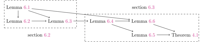
In this section, we will prove Theorem4.1. For that purpose, we build a quite amount of preparation material in sections 6.1 to 6.3 before we prove the theorem in section 6.4. Figure 6.1 shows a pictorial description of our proof process.
Lemma6.1
Lemma6.2 Lemma 6.3 Lemma6.4 Lemma6.6
Lemma6.5 Theorem4.1
section6.2
section6.3
Figure 6.1: Proof process for Theorem4.1
6.1
Simplification
Without loss of generality, we may assume that the covariance matrixΣdiagonal. Otherwise, we can perform a (constant) orthogonal transformation as follows. Recall the spectral decomposition
Σ=U ΛUT in (3.1). Instead of the random vectorX, we equivalently consider
Y ≡[Y1,Y2, . . . ,Yn]T:=UTX.
Accordingly, perform the same orthogonal transformation on all involved quantities:
Y(n)=UTX(n), V(n)=UTU(n), V
∗=UTU∗=
Ip 0
As consequences, we will have the equivalent versions of Algorithm3.1, Theorems4.1,4.2and4.3. Firstly, because
(V(n−1))TY(n)= (U(n−1))TX(n), (Y(n))TY(n)= (X(n))TX(n),
the equivalent version of Algorithm 3.1 is obtained by symbolically replacing all letters X, U by
Y, V while keeping their respective superscripts. If the algorithm converges, it is expected that
R(V(n))
→ R(V∗). Secondly, noting
kΣ−1/2Xkψ2 =kU Λ−
1/2UT
Xkψ2 =kΛ−
1/2
Ykψ2,
we can restate Assumptions4.1and4.2equivalently as
(A-1′) E{Y}= 0,EnY YTo=Λ= diag(λ
1, . . . , λd) with (3.2);
(A-2′) ψ:=kΛ−1/2Y
kψ2 ≤ ∞.
(A-3′) k(Id−Π V∗)Yk
2
2 ≤(ν−1)pmax
kYk2
∞, λ1 , where 1 ≤ν is a constant, independent of d,
andV∗=R(V∗).
Thirdly, all canonical angles between two subspaces are invariant under the orthogonal transforma-tion. Therefore the equivalent versions of Theorems4.1,4.2and4.3forY is also simply obtained by replacing all lettersX, U byY, V while keeping their respective superscripts.
In the rest of this section, we will prove the mentioned equivalent version of Theorem 4.1. Likewise in the next section, we will prove the equivalent versions of Theorems4.2and4.3. In the other words, essentially we assume thatΣis diagonal.
To facilitate our proof, we introduce new notations for two particular submatrices of anyV ∈
Rd×p:
¯
V =V(1:p,:),
¯
V =V(p+1:d,:). (6.2)
In particular,T(V) =
¯
VV¯−1 for the operatorT defined in (2.3), provided ¯V is nonsingular. Set
¯
Λ= diag(λ1, . . . , λp),
¯
Λ= diag(λp+1, . . . , λd). (6.3)
Although the assignments to ¯Λand ¯
Λare not consistent with the extractions defined by (6.2), they don’t seem to cause confusions in our later presentations.
Forκ >1, defineS(κ) :={V ∈Rd×p:σ( ¯V)⊂[1
κ,1]}. It can be verified that
V ∈S(κ)⇔ kT(V)k2≤pκ2−1. (6.4)
For the sequenceV(n), define
Nout{S(κ)}:= min{n:V(n)∈/ S(κ)}, Nin{S(κ)}:= min{n:V(n)∈S(κ)}.
Nout{S(κ)}is the first step of the iterative process at whichV(n)jumps fromS(κ) to outside, and
Nin{S(κ)}is the first step of the iterative process at whichV(n)jumps from outside toS(κ). Also,
define e
λ:=λ1β−2ε, Nqb{eλ}:= min
n
n≥1 : max{kY(n)
k∞,kZ(n)k∞} ≥eλ1/2 o
.
Nqb{eλ}is the first step of the iterative process at which an entry of Y(n) orZ(n)exceedsλe. For
n < Nqb{eλ}, we have
kY(n)k2<(deλ)1/2, kZ(n)k2<(peλ)1/2.
Moreover, under (A-3′),kY(n)
k2<(νpλe)1/2.
For convenience, we will set T(n)=T(V(n)), and letF
n =σ{Y(1), . . . , Y(n)}be theσ-algebra filtration, i.e., the information known by step n. Also, since in this section ε, β are fixed, we suppress the dependency information ofM(ε) on εand Ns = Ns(β) onβ to simply write M =
Lastly, we discuss some of the important implications of the condition
0< β <min 1,
√
2−1
νpλ1
! 1
1−2ε
,
1 8κpλ1
2
1−4ε
,
γ2
130ν1/2κ2p2λ2 1
1
ε
. (4.6b)
It guarantees that
(β-1) β <1 andβγ=β1/2+2εβ1/2−2ε(λ
p−λp+1)≤8κpλ1 1λ1≤161√3;
(β-2) dβeλ≤β2εωλ
1β−2ε≤ωλ1;
(β-3) pβeλ≤νpβeλ=νpλ1β1−2ε≤√2−1.
Set
CV =5 2 +
7
2(νpλβe ) + 15
8 (νpeλβ)
2+3
8(νpeλβ)
3
≤16 + 13 √
2
8 ≈4.298; (6.5a)
C∆= 2 + 1
2(νpeλβ) +CVpeλβ≤
22 + 7√2
8 ≈3.987; (6.5b)
CT =CV + 2C∆+ 2C∆CVpeλβ≤
251 + 122√2
16 ≈26.471; (6.5c)
Cκ=
(3−√2)C2
∆ 64(CT+ 2C∆)2 ≤
565 + 171√2
21504 ≈0.038; (6.5d)
Cν = 4√2CTCκ≤223702 + 183539
√
2
86016 ≈5.618; (6.5e)
C◦= 29 + 8
√
2 16(3−√2) +
4CT (3−√2)C∆
β3ε+ [CT +29 + 8
√
2 32 ]β
1/2−3ε
+ 3C
2
T 2(3−√2)C2
∆
β1/2+3ε+2CT
C∆
β1−3ε+ C
2
T 2C2
∆
β3/2−3ε
≤2582968 + 1645155 √
2
14336 ≈342.464. (6.5f)
The condition (4.6b) also guarantees that
(β-4) 2C∆peλβ1/2κ= 2C∆pλ1β1/2−2εκ≤ 2C8∆ <1, and thus 2C∆peλβκ <1;
(β-5) 4√2CTν1/2κ2p2λe2γ−1β5ε ≤1, and thus 4√2CTν1/2κ2p2eλ2γ−1β1/2+χ ≤1 for χ ∈[−1/2 + 5ε,0].
6.2
Increments of One Iteration
Lemma 6.1. For any fixedK≥1,
PnNqb{eλ}> K
o
≥1−e(d+p)Kexp(−Cψψ−1β−2ε),
whereCψ is an absolute constant.
Proof. Since n
Nqb{eλ} ≤K
o
⊂ [
n≤K n
kY(n)
k∞≥eλ1/2 o
∪nkZ(n)
k∞≥eλ1/2 o
⊂ [
n≤K
[
1≤i≤d n
|eT
i Y(n)| ≥eλ1/2 o
∪ [
1≤j≤p n
|eT
jZ(n)| ≥eλ1/2 o
= [
Proof. To avoid the cluttered superscripts, in this proof, we drop the superscript “·(n)” and use
the superscript “·+” to replace “
By Taylor’s expansion, there exists 0< ξ < αsuch that
whereR=−β
2
2 (Z
TZ)(2 +βYTY)Y +ζβ2(ZTZ)V Z+ζβ3(ZTZ)2Y for which
kRk2≤
β2
2 (peλ)(2 +βνpeλ)(νpλe)
1/2+ζβ2(peλ)3/2+ζβ3(peλ)2(νpλe)1/2
=
1
2(2 +βνpeλ) + 3
8(2 +βνpλe)
2+3
8(2 +βνpeλ)
2(βpeλ)
ν1/2(peλ)3/2β2
=CVν1/2(peλ)3/2β2, as expected.
Lemma 6.3. Suppose that the conditions of Theorem4.1hold. Let τ=kT(n)
k2, andCT be as in (6.5c). Ifn <minnNqb{λe}, Nout{S(κ)}
o
, then the following statements hold.
1. T(n) andT(n+1) are well-defined.
2. DefineET(n)(V(n))by E
T(n+1)−T(n)F
n =β( ¯
ΛT(n)−T(n)Λ¯) +E(n)
T (V(n)). Then
(a) supV∈S(κ)kE (n)
T (V)k2≤CTν1/2(peλβ)2(1 +τ2)3/2;
(b) kT(n+1)
−T(n)
k2≤ν1/2(peλβ)(1 +τ2) +CTν1/2(peλβ)2(1 +τ2)3/2.
3. DefineR◦ by var◦ T(n+1)
−T(n)
|Fn
=β2H
◦+R◦. Then
(a) H◦= var◦ Y¯Y¯T≤16ψ4H, whereH = [ηij](d−p)×pwithηij=λp+iλj fori= 1, . . . , d−
p,j= 1, . . . , p;
(b) kR◦k2≤(νpλβe )2τ(1 +112τ+τ2+14τ3) + 4CTν(pλβe )3(1 +τ2)5/2+ 2CT2ν(pλβe )4(1 +τ2)3.
Proof. For readability, we will drop the superscript “·(n)”, and use the superscript “
·+” to replace
“·(n+1)” forV, R, drop the superscript “
·(n+1)” onY, Z, and drop the conditional sign “
|Fn” in the computation of E{·},var(·),cov(·) with the understanding that they are conditional with respect toFn. Finally, for any expression or variableF, we define∆F :=F+
−F.
Consider item 1. Sincen < Nout{S(κ)}, we haveV ∈S(κ) andτ =kTk2≤(κ2−1)1/2. Thus,
kV¯−1k2≤κandT =
¯
VV¯−1 is well-defined. Recall (6.6) and the partitioning
Y =
1
p Y¯
d−p ¯
Y
, R=
1
p R¯
d−p ¯
R
.
We have∆V¯ =β( ¯Y ZT−(1 + β
2YTY) ¯V ZZT) + ¯RZT, and
¯
R=−β
2
2 (Z
TZ)(2 +βYTY) ¯Y +ζβ2(ZTZ) ¯V Z+ζβ3(ZTZ)2Y .¯
NoticingkY¯k2≤(peλ)1/2, we find
k∆V¯k2≤β(peλ) +β(1 +β
2νpeλ)peλ+CV(peλ)
2β2
≤
2 + β
2νpλe+CVpeλβ
peλβ=C∆peλβ,
where C∆ is as in (6.5b). Thus k∆V¯V¯−1k2 ≤ k∆V¯k2kV¯−1k2 ≤C∆peλβκ ≤1/2 by (β-4). As a result, ¯V+ is nonsingular, and
k( ¯V+)−1k2≤ k
¯
V−1k2
1− kV¯−1∆V¯k2 ≤
In particular,T+=
¯
V+( ¯V+)−1 is well-defined. This proves item1.
For item2, using the Shermann-Morrison-Woodbury formula [5, p. 95], we get
∆T = ¯
V+( ¯V+)−1− ¯
VV¯−1
= ( ¯
V +∆
¯
V)( ¯V +∆V¯)−1−V¯V¯−1
= ( ¯
V +∆
¯
V)( ¯V−1−V¯−1∆V¯( ¯V +∆V¯)−1)− ¯
VV¯−1
=∆
¯
VV¯−1−
¯
VV¯−1∆V¯( ¯V +∆V¯)−1−∆
¯
VV¯−1∆V¯( ¯V +∆V¯)−1 =∆
¯
VV¯−1−¯VV¯−1∆V¯( ¯V−1−V¯−1∆V¯( ¯V +∆V¯)−1)−∆
¯
VV¯−1∆V¯( ¯V +∆V¯)−1 =∆
¯
VV¯−1−T ∆V¯V¯−1+T ∆V¯V¯−1∆V¯( ¯V+)−1−∆
¯
VV¯−1∆V¯( ¯V+)−1 = [∆
¯
V −T ∆V¯][I−( ¯V+)−1∆V¯] ¯V−1.
WriteTL=−T I andTR=
I T
, and thenTLV = 0 andV =TRV¯. Thus,
∆T =TL∆V[I−( ¯V+)−1∆V¯]VTTR. Since∆V is rank-1,∆T is also rank-1. By Lemma6.2,
∆T =TL
βY ZT
−β(1 +β 2Y
TY)V ZZT+RZT
I−( ¯V+)−1∆V¯VTT
R
=TLβY YTV +RZT I−( ¯V+)−1∆V¯VTTR =TL(βY YTV VT+R
T)TR
=TL(βY YT+RT)TR,
(6.7)
whereRT =RZTVT−(βY +R)ZT( ¯V+)−1∆V V¯ T.Note that
TLY YTTR= ¯
YY¯T−TY¯
¯
YTT−TY¯Y¯T+ ¯
Y
¯
YTT, (6.8)
and
E ¯
YY¯T = 0, ETY¯Y¯T =TEY¯Y¯T =TΛ,¯ (6.9a) ETY¯
¯
YTT =TEY¯
¯
YT T = 0, E ¯
Y
¯
YTT = E ¯
Y
¯
YT T = ¯
ΛT, (6.9b)
Thus, E{∆T}=β( ¯
ΛT −TΛ¯) +ET(V), whereET(V) = E{TLRTTR}. SinceV ∈S(κ),kTk2≤(κ2−1)1/2by (6.4). Thus
kRTk2≤ kRk2(peλ)1/2+ [(νpeλ)1/2β+kRk2](peλ)1/22(1 +kTk22)1/2C∆peλβ
≤CVν1/2(peλ)2β2+ (1 +kTk22)1/2[1 +CVpλβe ]2C∆ν1/2(peλ)2β2
≤CTν1/2(peλβ)2(1 +kTk22)1/2,
(6.10)
whereCT =CV + 2C∆(1 +CVpλβe ). Therefore,
kET(V)k2≤E{kTLRTTRk2} ≤(1 +kTk22) E{kRTk2}.
Item2(a)holds. For item2(b), we have
k∆Tk2≤(1 +kTk22)(βkY YTV VTk2+kRTk2)
≤β(νpeλ)1/2(pλe)1/2(1 +kTk2
2) +CTν1/2(pλβe )2(1 +kTk22)3/2
≤ν1/2peλβ(1 +kTk2
2) +CTν1/2(peλβ)2(1 +kTk22)3/2.
Now we turn to item3. We have
whereR◦,1= cov◦ TLY YTTR, TLRTTR, andR◦,2= var◦(TLRTTR). By (6.8),
var◦ TLY YTTR= var◦ Y¯Y¯T+R◦,0, (6.12)
where
R◦,0= var◦ TY¯¯YTT
+ var◦ TY¯Y¯T+ var◦ ¯
Y
¯
YTT
−2 cov◦ ¯
YY¯T, TY¯
¯
YTT−2 cov◦ ¯
YY¯T, TY¯Y¯T+ 2 cov◦ ¯
YY¯T,
¯
Y
¯
YTT
+ 2 cov◦ TY¯
¯
YTT, TY¯Y¯T−2 cov◦ TY¯
¯
YTT,
¯
Y
¯
YTT−2 cov◦ TY¯Y¯T,
¯
Y
¯
YTT.
Examine (6.11) and (6.12) together to get H◦ = var◦ ¯
YY¯T and R◦ =β2R
◦,0+ 2βR◦,1+R◦,2.
We note
Yj =eTjY =eTjΛ1/2Λ−1/2Y =λ
1/2
j eTjΛ−1/2Y,
eTi var◦ Y¯Y¯T
ej= var(eTi ¯YY¯Tej) = var(Yp+iYj) = E
Yp2+iYj2 . By [20, (5.11)],
EYj4 =λ2jE n
(eTjΛ−1/2Y)4 o
≤16λ2jkeTjΛ−1/2Yk4ψ2 ≤16λ
2
jkΛ−1/2Yk4ψ2= 16λ
2
jψ4. Therefore
eTi var◦ ¯YY¯T
ej≤[E
Yp4+i E
Yj4 ]1/2≤16λp+iλjψ4, i.e., H◦ = var◦ ¯YY¯T
≤16ψ4H. This proves item 3(a). To show item3(b), first we bound the entrywise variance and covariance. For any matrices A1, A2, by Schur’s inequality (which was
generalized to all unitarily invariant norm in [6, Theorem 3.1]),
kA1◦A2k2≤ kA1k2kA2k2, (6.13)
we have
kcov◦(A1, A2)k2=kE{A1◦A2} −E{A1} ◦E{A2}k2
≤E{kA1◦A2k2}+kE{A1} ◦E{A2}k2
≤E{kA1k2kA2k2}+kE{A1}k2kE{A2}k2, (6.14a)
kvar◦(A1)k2≤E
kA1k22 +kE{A1}k22. (6.14b)
Apply (6.14) toR◦,1 andR◦,2 to get
kR◦,1k2≤2CTν(pλe)3β2(1 +kTk22)5/2, kR◦,2k2≤2CT2ν(peλβ)4(1 +kTk22)3, (6.15)
upon using
kTLY YTTRk2=kTLY YTV VTTRk2≤ν1/2(pλe)(1 +kTk22),
kTLRTTRk2≤CTν1/2(peλβ)2(1 +kTk22)3/2.
ForR◦,0, by (6.9), we have
kcov◦ Y¯Y¯T, TY¯¯YTTk2≤Ek
¯
YY¯Tk22 kTk22,
kcov◦ ¯YY¯T, TY¯Y¯Tk2≤Ek
¯
YY¯Tk2kY¯Y¯Tk2 kTk2,
kcov◦ ¯YY¯T,¯Y¯YTTk2≤Ek
¯
YY¯Tk2k
¯
Y
¯
YTk2 kTk2,
kcov◦ TY¯¯YTT, TY¯Y¯Tk2≤Ek
¯
YY¯Tk2kY¯Y¯Tk2 kTk32,
kcov◦ TY¯¯YTT,Y¯¯YTTk2≤Ek
¯
YY¯Tk2k
¯
Y
¯
YTk2 kTk32,
kvar◦ TY¯¯YTTk2≤Ek
¯
kvar◦ TY¯Y¯Tk2≤EkY¯Y¯Tk22 kTk22+kTΛ¯k22,
6.3
Quasi-power iteration process
DefineD(n+1)=T(n+1)
norm induced by the matrix normk·kui. Recursively,
Lemma 6.4. Suppose that the conditions of Theorem4.1hold. Ifn <minnNqb{eλ}, Nout{S(κβχ)}
o
andV(0)
∈S(κβχ), then for any χ
∈(5ε−1/2,0]andκ >√2, we have
P{Mn(χ+ 1/2)} ≥1−2dexp(−Cκγκ−2ν−1p−2λ1−2β−2ε), (6.20)
whereCκ is as in (6.5d).
Proof. Sinceκ >√2, we haveκ2β2χ >2 andκβχ<[2(κ2β2χ−1)]1/2. Thus, by (β-5),
4CTν1/2κ3p2eλ2γ−1β1+3χ(κ2β2χ−1)−1/2β−1/2−χ≤4
√
2CTν1/2κ2p2λe2γ−1β1/2+χ≤1.
For any n < minnNqb{eλ}, Nout{S(κβχ)}
o , V(n)
∈ S(κβχ) and thus
kT(n)
k2 ≤
p
κ2β2χ−1 by (6.4). Therefore, by item2(b)of Lemma 6.3, we have
kD(n+1)k2=
T(n+1)−T(n)−EnT(n+1)−T(n)Fno
2
≤ kT(n+1)−T(n)k2+ E
n
kT(n+1)−T(n)k2
Fn
o
≤2ν1/2peλβ(1 +
kT(n)
k2
2)[1 +CTpeλβ(1 +kT(n)k22)1/2]
≤2κ2ν1/2pλβe 1+2χ[1 +C
Tκpeλβ1+χ].
(6.21)
For anyn <minnNqb{eλ}, Nout{S(κβχ)}
o ,
kJ3k2≤
n X
s=1
kLkn2−skE (s−1)
T (V
(s−1))
k2
≤CTν1/2κ3(peλ)2β2+3χ n X
s=1
(1−βγ)n−s
≤CTν
1/2κ3(peλ)2β2+3χ
βγ =CTν
1/2κ3(pλe)2γ−1β1+3χ
≤14(κ2β2χ−1)1/2β1/2+χ.
Similarly,
kJ2k2≤
n X
s=1
kLkn−s
2 kD(s)k2
≤ 2κ
2ν1/2pλβe 2χ(1 +C
Tκpeλβ1+χ)
γ
≤ 2κ
2ν1/2peλβ2χ
γ +
1 2(κ
2β2χ
−1)1/2β1/2+χ.
Also,kJ1k2≤ kLkn2kT(0)k2≤ kT(0)k2≤(κ2β2χ−1)1/2. For fixedn >0 andβ >0,
M
(n) 0 :=L
nT(0), M(n)
t :=LnT(0)+
min{t,NoutX{S(κ)}−1}
s=1
Ln−sD(s):t= 1, . . . , n
forms a martingale with respect toFt, because
EnkMt(n)k2
o
≤ kJ1k2+kJ2k2<+∞,
and
EnMt(+1n)−M (n)
t Ft
o
= EnLn−t−1D(t+1)
Ft o
=Ln−t−1EnD(t+1)
Ft o
Use the matrix version of Azuma’s inequality [18, Section 7.2] to get, for anyα >0,
PnkM(n)
n −M
(n) 0 k2≥α
o
≤2dexp(−α
2
2σ2),
where
σ2=
min{n,NoutX{S(κ)}−1}
s=1
kLn−sD(s)k22
≤[2κ2ν1/2peλβ1+2χ(1 +C
Tκpeλβ1+χ)]2
min{n,NoutX{S(κ)}−1}
s=1
(1−βγ)2(n−s)
≤4κ
4νp2eλ2β2+4χ(1 +C
Tκpλβe 1+χ)2
βγ[2−βγ]
≤4κ
4νp2eλ2γ−1β1+4χ(1 + CT
2C∆)
2
3−√2 by (β-4),eλβ
1/2
≤2κpC1
∆
=Cσκ4νp2γ−1eλ2β1+4χ,
andCσ=(CT+2C∆)
2
(3−√2)C2
∆. Thus, noticingJ2=M
(n)
n −M0(n) forn≤Nout{S(κ)} −1, we have
P{kJ2k2≥α} ≤2dexp
− α
2
2Cσκ4νp2γ−1eλ2β1+4χ
.
Choosing α = 1 4(κ
2β2χ
−1)1/2βχ+1/2−3ε and noticing
kJ3k2 ≤ 14(κ2β2χ −1)1/2βχ+1/2−3ε and
T(n)
− LnT(0)=J
2+J3, we have
P{Mn(χ+ 1/2)c}= P
kT(n)− LnT(0)k2≥
1 2(κ
2β2χ
−1)1/2βχ+1/2−3ε
≤P
kJ2k2≥
1 4(κ
2β2χ
−1)1/2βχ+1/2−3ε
≤2dexp
− κ
2β2χ
−1 32Cσκ4νp2γ−1eλ2β2χ
β−6ε
≤2dexp
− κ
2β2χ 64Cσκ4νp2γ−1eλ2β2χ
β−6ε
= 2dexp(−Cκγκ−2ν−1p−2λ−12β−2ε),
whereCκ=641Cσ which is the same as in (6.5d).
Lemma 6.5. Suppose that the conditions of Theorem 4.1hold. If
N2−m(1−6ε)<min n
Nqb{λe}, Nout{S(κβχ)}
o
andV(0)∈S(β(1−21−m
)(3ε−1/2)κ
m/2)with m≥2, then for κm>√2
P{Hm} ≥1−2dN2−m(1−6ε)exp(−Cκγκ−m2ν−1p−2λ−12β−2ε),
whereHm= n
Nin
n
S(p3/2β(1−22−m
)(3ε−1/2)κm)o≤N
2−m(1−6ε) o
.
Proof. By the definition of the eventTn,
Tn(2−m[1−6ε] + 3ε) =nkT(n)k2≤(κ2m−β(1−2
1−m)(1
Forn≥N2−m(1−6ε)and V(0)∈S(β(1−2
1−m)(3ε
−1/2)κ
m/2),
Mn(2−m(1−6ε) + 3ε)⊂Tn(2−m(1−6ε) + 3ε)
because
kT(n)k2≤ kT(n)− LnT(0)k2+kLkn2kT(0)k2
≤12κ2m−β(1−2
1−m)(1
−6ε)1/2β(1−22−m)(3ε −1/2)
+β2−m(1−6ε)κ
2
m 4 −β
(1−21−m)(1
−6ε)1/2β(1−21−m)(3ε −1/2)
≤κ2m−β(1−2
1−m)(1
−6ε)1/2β(1−21−m)(3ε −1/2).
Therefore, noticing
κ2m−β(1−2
1−m)(1
−6ε)1/2β(1−22−m)(3ε
−1/2)=β(1−22−m)(6ε −1)κ2
m−β2
1−m(1
−6ε)1/2
≤32β(1−22−m)(6ε−1)κ2m−1 1/2
,
we get
MN2−m(1−6ε)(2
−m(1
−6ε) + 3ε)⊂nNin
n
S(p3/2β(1−22−m)(3ε−1/2)κm)o≤N2−m(1−6ε) o
=:Hm.
Since
\
n≤minnN2−m(1−6ε),Nin
n
S(√3/2β(1−22−m)(3ε−1/2)κm)o−1o
Mn(2−m(1
−6ε) + 3ε)∩Hcm
⊂ \
n≤N2−m(1−6ε)
Mn(2−m(1−6ε) + 3ε)⊂MN2−m(1−6ε)(2
−m(1
−6ε) + 3ε),
we have
\
n≤minnN2−m(1−6ε),Nin
n
S(√3/2β(1−22−m)(3ε−1/2)κm)o−1o
Mn(2−m(1
−6ε) + 3ε)⊂Hm.
By Lemma6.4withχ= 2−m(1
−6ε) + 3ε−1 2 = 2−
m(1
−2m−1)(1
−6ε), we get
P{Hcm} ≤P
[
n≤minnN2−m(1−6ε),Nin
n
S(√3/2β(1−22−m)(3ε−1/2)κ
m) o
−1o
Mn(2−m(1−6ε) + 3ε)c
≤minnN2−m(1−6ε), Nin n
S(p3/2β(1−22−m)(3ε−1/2)κm)o−1o
×2dexp(−Cκγκ−m2ν−1p−2λ−12β−2ε)
≤2dN2−m(1−6ε)exp(−Cκγκm−2ν−1p−2λ−12β−2ε), as expected.
Lemma 6.6. Suppose that the conditions of Theorem 4.1 hold. IfV(0)
∈S(κ/2) with κ >2√2, K > N1−6ε, then there exists a high-probability event H1∩QK = Tn∈[N1/2−3ε,K]Tn(1/2)∩QK
satisfying
such that for anyn∈[N1−6ε, K],
EnT(n)◦T(n); H1∩QK o
≤ L2nT(0)◦T(0)+ 2β2[I− L2]−1[I− L2n]H◦+RE,
where kREk2 ≤ C◦κ4γ−1ν2(pλe)2β3/2−3ε, H◦ = var◦ ¯YY¯T
≤ 16ψ4H is as in item 3(a) of
Lemma6.3, and C◦ is as in (6.5f).
Proof. First we estimate the probability of the eventH1. We knowTn(1/2)⊂kT(n)k2≤(κ2−1)1/2 .
IfK≥Nout{S(κ)}, then there exists somen≤K, such thatV(n)∈/S(κ), i.e.,kT(n)k2>(κ2−1)1/2
by (6.4). Thus,
{K≥Nout{S(κ)}} ⊂
[
n≤K n
kT(n)k2>(κ2−1)1/2
o
⊂ [
n≤K
Tn(1/2)c.
On the other hand, forn≥N1/2−3ε andV(0)∈S(κ/2), Mn(1/2)⊂Tn(1/2) because
kT(n)
k2≤ kT(n)− LnT(0)k2+kLkn2kT(0)k2
≤ 12(κ2−1)1/2β1/2−3ε+β1/2−3εκ
2
4 −1 1/2
≤(κ2
−1)1/2β1/2−3ε. (6.22) Therefore,
\
n∈[N1/2−3ε,K]
Mn(1/2)⊂ \ n∈[N1/2−3ε,K]
Tn(1/2)⊂ {K≤Nout{S(κ)} −1},
and so
\
n≤min{K,Nout{S(κ)}−1}
Mn(1/2)⊂ \
n∈[N1/2−3ε,min{K,Nout{S(κ)}−1}]
Mn(1/2)
= \
n∈[N1/2−3ε,K]
Mn(1/2)
⊂ \
n∈[N1/2−3ε,K]
Tn(1/2)
=:H1.
By Lemma6.4withχ= 0, we have
P
[
n≤min{K,Nout{S(κ)}−1}
Mn(1/2)c∩QK
≤min{K, Nout{S(κ)} −1} ·2dexp(−Cκγκ−2ν−1p−2λ−12β−2ε)
= 2dKexp(−Cκγκ−2ν−1p−2λ−12β−2ε).
Thus, by Lemma6.1,
P{(H1∩QK)c}= P{Hc1∪QcK}
= P{Hc1∩QK}+ P{QcK}
≤P
[
n≤min{K,Nout{S(κ)}−1}
Mn(1/2)c∩QK + P{Q
c
K}
Next we estimate the expectation. Since
H1=
\
n∈[N1/2−3ε,K]
Tn(1/2)⊂ \
n∈[N1/2−3ε,K] n
1Tn−1D
(n)=D(n)o,
we have forn∈[N1/2−3ε, K]
T(n)1H1∩QK =1QK
LnT(0)+
N1/2−3ε−1
X
s=1
Ln−sD(s)+
n X
s=N1/2−3ε
Ln−sD(s)1
Ts−1+
n X
s=1
Ln−sE(s−1)
T (V
(s−1))
=:J1+J21+J22+J3.
In what follows, we simply writeET(n)=ET(n)(V(n)) for convenience. Then,
EnT(n)◦T(n); H1∩QK o
= EnT(n)◦T(n)1H1∩QK o
= E{J1◦J1}+ 2 E{J1◦J21}+ 2 E{J1◦J22}+ 2 E{J1◦J3}
+ E{[J21+J22]◦[J21+J22]}+ 2 E{[J21+J22]◦J3}+ E{J3◦J3}
≤E{J1◦J1}+ 2 E{J1◦J21}+ 2 E{J1◦J22}+ 2 E{J1◦J3}
+ 2 E{J21◦J21}+ 4 E{J21◦J22}+ 2 E{J22◦J22}+ 2 E{J3◦J3}.
In the following, we estimate each summand above forn∈[N1−6ε, K]. We have the following. 1. E{J1◦J1}=L2nT(0)◦T(0).
2. E{J1◦J21}=
N1/X2−3ε−1
s=1
L2n−sT(0)◦EnD(s)1QK o
= 0, because
EnD(s)1QK o
= EnEnD(s)1QK Fs−1
oo = 0.
3. E{J1◦J22}=
n X
s=N1/2−3ε
L2n−sT(0)
◦EnD(s)1Ts−11QK o
= 0, becauseTs−1⊂Fs−1and so
EnD(s)1Ts−11QK o
= P{Ts−1}E
n
D(s)1QK Ts−1
o
= P{Ts−1}E
n
EnD(s)1
QK
Fs−1o Ts−1
o = 0.
4. E{J1◦J3}=
n X
s=1
L2n−sT(0)◦EnET(s−1)1QK o
. Recall (6.13). By item2(a)of Lemma6.3, we
have
kE{J1◦J3}k2≤
n X
s=1
kLk22n−skT(0)k2kE
n
ET(s−1)1QK o
k2
≤
n X
s=1
(1−βγ)2n−s(κ
2
4 −1)
1/2C
Tν1/2(peλβ)2κ3
≤(1−βγ)n(κ2−1)1/2CTν1/2p2eλ2β2κ3 2βγ
≤(1−βγ)
2(n+1−N1/2−3ε)
βγ[2−βγ] E{kR◦k2}
≤12−βγ −βγ
(1−βγ)n
βγ E{kR◦k2}
≤12β1−6εγ−1βκ4ν(peλ)2 29 + 8
√
2
32 ν+ 4CTκ(peλβ) + 2C
2
Tκ2(peλβ)2 !
≤ 29 + 8 √
2
64 + 2CTκ(pλβe ) +C
2
Tκ2(peλβ)2 !
γ−1κ4ν2(peλ)2β2−6ε.
7. For E{J22◦J22}, we have
E{J22◦J22}=
n X
s=N1/2−3ε
L2(n−s)EnD(s)1QK1Ts−1◦D
(s)1
QK1Ts−1
o
=β2
n X
s=N1/2−3ε
L2(n−s)H◦+ n X
s=N1/2−3ε
L2(n−s)ER◦1Ts−1 ,
because fors6=s′,
EnD(s)1QK1Ts−1◦D
(s′)
1QK1Ts′−1
o
= EnD(s)◦D(s′)1QK1Ts−11Ts′−1
o
= P{Ts−1∩Ts′−1}E
n
D(s)◦D(s′)1QK
Ts−1∩Ts′−1
o
= P{Ts−1∩Ts′−1}E
n
EnD(max{s,s′})1QK
Fmax{s,s′}−1
o
◦D(min{s,s′})Ts−1∩Ts′−1
o
= 0,
and
EnD(s)1
QK1Ts−1◦D
(s)1
QK1Ts−1
o
= EnD(s)
◦D(s′)
1QK1Ts−1
o
= P{Ts−1}E
n EnD(s)
◦D(s)1
QK
Fs−1o Ts−1
o
≤β2H◦+ ER◦1Ts−1 .
We have
kR◦1Ts−1k2≤
29 + 8√2 32 κ
3ν2(peλβ)2τ
s−1+ 4CTκ5ν(peλβ)3+ 2CT2κ6ν(peλβ)4
≤29 + 8 √
2 32 κ
3ν2(peλβ)2(κ2
−1)1/2β1/2−3ε+ 4C
Tκ5ν(peλβ)3+ 2CT2κ6ν(peλβ)4
≤29 + 8 √
2 32 κ
4ν2(peλβ)2β1/2−3ε+ 4C
Tκ5ν(peλβ)3+ 2CT2κ6ν(peλβ)4.
WriteE22:=
n X
s=N1/2−3ε
L2(n−s)ER◦1Ts−1 for which we have
kE22k2≤
n X
s=N1/2−3ε
kLk2(2n−s)E
kR◦1Ts−1k2
≤βγ[21 −βγ]E
kR◦1Ts−1k2
≤ 1
3−√2γ
−1κ4ν(peλ)2β 29 + 8
√
2 32 νβ
1/2−3ε+ 4C
≤ 1
Collecting all estimates together, we obtain
EnT(n)◦T(n); H1∩QK
6.4
Proof of Theorem
4.1
Writeκm= 6(1−m)/2κform= 1, . . . , M ≡M(ǫ). Sincedβ1−7ε≤ω, we know
φd1/2≤φω1/2β7ε/2−1/2≤β(1−21−M)(3ε−1/2)κM/2.
The key to our proof is to divide the whole process intoM segments of iterations. Thanks to the strong Markov property of the process, we can use the final value of current segment as the initial guess of the very next one. By Lemma6.5, after the first segment of
n1:= min
n
Nin
n
S(p3/2β(1−22−M
)(3ε−1/2)κ 1)
o
, N2−M(1−6ε) o
iterations,V(n1) lies in S(p3/2β(1−22−M)(3ε−1/2)κ
1) =S(β(1−2
2−M)(3ε
−1/2)κ
2/2) with high
prob-ability, which will be a good initial guess for the second segment. In general, theith segment of iterations starts withV(ni−1) and ends withV(ni), where
ni= min (
Nin
n
S(β(1−2i+1−M)(3ε−1/2)κi+1/2)
o
,
& M X
m=M+1−i e
N2−m(1−6ε) ')
.
At the end of the (M −1)st segment of iterations, V(nM−1) is produced and it is going to be
used as an initial guess for the last step, at which we can apply Lemma 6.6. Now nM−1 =
minnNin{S(κM/2)},Kb o
, where Kb = lPMm=2Ne2−m(1−6ε) m
= lNe(1−21−M)(1/2−3ε) m
. By 22−M
≥
ε/2
1/2−3ε ≥21−M, we have
N1/2−7ε/2=
l e
N1/2−7ε/2
m
≤Kb ≤lNe1/2−13ε/4
m
≤N1/2−13ε/4.
Let
e
Hm= n
Nin
n
S(p3/2β(1−22−m
)(3ε−1/2)κ
M+1−m) o
≤Ne2−m(1−6ε)+nM−m o
form= 2, . . . , M ,
e
H1=
\
n∈[N1/2−3ε,K−Nin{S(κM/2)}]
Tn+Nin{S(κM/2)}(1/2),
H= M \
m=1
e
Hm∩QK,
wheren0= 0. We have
P{Hc}= P
( M
[
m=1
e
Hcm∪QcK
)
≤
M X
m=1
PnHecm∪QcKo
≤
M X
m=2
2dN2−m(1−6ε)exp(−Cκγκ−2
M+1−mν−
1p−2λ−2 1 β−2ε)
+ 2dK−
M X
m=2
N2−m(1−6ε)
exp(−Cκγκ−M2ν−
1p−2λ−2 1 β−
2ε)
+ eK(d+p) exp −Cψψ−1β−2ε
≤2dKexp(−Cκγκ−2ν−1p−2λ−12β−2ε) + eK(d+p) exp −Cψψ−1β−2ε
≤2dKexp(−Cκ4√2CTν−1/2βεβ−2ε) + eK(d+p) exp −Cψψ−1β−εβ−ε
by (β-5)
≤2dKexp(−4√2CTCκν−1/2β−ε) + eK(d+p) exp −Cψψ−1β−ε
≤K[(2 + e)d+ ep] exp(−max{Cνν−1/2, Cψψ−1}β−ε),