INDOOR POSITIONING BY VISUAL-INERTIAL ODOMETRY
M. Ramezani *, D. Acharya, F. Gu, K. Khoshelham
Department of Infrastructure Engineering, The University of Melbourne, Parkville 3010 Australia (mramezani, acharyad, fuqiangg)@student.unimelb.edu.au, [email protected]
KEY WORDS: Visual-Inertial Odometry, Kalman Filter, Omnidirectional Cameras, Inertial Measurements, Indoor Positioning
ABSTRACT:
Indoor positioning is a fundamental requirement of many indoor location-based services and applications. In this paper, we explore the potential of low-cost and widely available visual and inertial sensors for indoor positioning. We describe the Visual-Inertial Odometry (VIO) approach and propose a measurement model for omnidirectional visual-inertial odometry (OVIO). The results of experiments in two simulated indoor environments show that the OVIO approach outperforms VIO and achieves a positioning accuracy of 1.1% of the trajectory length.
1. INTRODUCTION
Robust and real-time indoor positioning is crucial in location-based services and applications such as indoor navigation, emergency response, and tracking goods inside buildings (Gu, et al., 2009). Since Global Navigation Satellite System (GNSS) signals are mostly blocked or jammed by obstacles such as walls and ceilings, or interfered by wireless equipment, GNSS cannot provide a reliable and continuous positioning solution in indoor environments. Consequently, various technologies for indoor positioning have been proposed in the past few years. Wireless technologies such as Wi-Fi, ZigBee, Bluetooth, Ultra-WideBand (UWB), and magnetic measurements have been used and tested by different industrial and research teams (Liu, et al., 2007). The Indoor Positioning Systems (IPSs) based on these technologies can estimate the position of a user or object at a course granularity, with accuracies in the order of tens of meters, up to a fine granularity, with accuracies down to a few meters (Konstantinidis, et al., 2015). However, these IPSs require an infrastructure of beacons and sensors pre-installed in the environment, which limits their applicability.
The common approach to infrastructure-free indoor positioning is Pedestrian Dead Reckoning (PDR). In PDR the position is estimated based on inertial measurements sensed by accelerometers and gyroscopes, which are available in most smartphones. The advantage of inertial positioning is that it is purely self-contained and therefore does not need any external references. In addition, inertial sensors can provide continuous positioning. However, due to the incremental nature of estimation in PDR, the position estimates drift over time (Groves, 2013). State of the art PDR approaches combine inertial measurements with step length estimation and use motion state recognition and landmarks to constrain the drift of position estimates (Gu, et al., 2016a; Gu, et al., 2016b).
Despite the widespread availability of cameras, e.g. on smartphones, they have mainly been used for positioning robots in indoor environments (Caruso, et al., 2015; Bonin-Font, et al., 2008). As an exteroceptive sensor, a camera captures visual information surrounding the user in a sequence of images, which can be matched to estimate the trajectory of the camera. This approach is usually referred to as Visual Odometry (VO) (Nistér, et al., 2004). The visual information can also be used to simultaneously construct a map of the environment, in an
approach commonly known as Simultaneous Localization and Mapping (SLAM) (Langelaan, 2007; Ong, et al., 2003). The accuracy of vision-based positioning can be better than 1 meter (Caruso, et al., 2015). However, using a camera as the only sensor for position estimation is likely to fail in environments with insufficient texture and geometric features, such as corridors with plain walls. To resolve this issue, visual information can be fused with inertial measurements. This approach is known as Visual-Inertial Odometry (VIO) (Mourikis & Roumeliotis, 2007; Kim & Sukkarieh, 2007; Li & Mourikis, 2013). In VIO, visual observations from a camera are fused with inertial measurements from an IMU within a filtering method such as an Extended Kalman Filter (EKF) to ensure continuous positioning in environments which lack salient features or texture.
Compared to perspective cameras, omnidirectional cameras such as dioptric cameras (with fish eye lens) and catadioptric cameras (with mirrors) provide a larger field of view (FoV) allowing image features to be tracked in longer sequences. This has been shown to result in more accurate position estimation (Zhang, et al., 2016). While omnidirectional cameras have been used in VO approaches (Caruso, et al., 2015; Zhang, et al., 2016), their performance within a VIO framework has not been evaluated for indoor positioning.
In this paper, we evaluate the performance of visual-inertial odometry using both perspective and omnidirectional cameras in simulated indoor environments. We fuse inertial measurements with image features tracked in multiple images within a Multi-State Constraint Kalman Filter (MSCKF) (Mourikis & Roumeliotis, 2007). We propose a new algorithm called Omnidirectional Visual-Inertial Odometry (OVIO) based on the MSCKF estimation approach. Because the standard perspective model is unsuited for omnidirectional cameras, in this algorithm, we define the measurement model on a plane tangent to the unit sphere rather than on the image plane.
The paper is organized as follows. In section 2, we briefly describe the visual-inertial odometry approach, and in Section 3 we propose a new algorithm to integrate omnidirectional images with inertial measurements. In section 4, we evaluate the performance of visual-inertial odometry in two simulated indoor environments. Finally, conclusions are drawn and directions for future research are discussed.
2. VISUAL-INERTIAL ODOMETRY USING A PERSPECTIVE CAMERA
Visual and inertial measurements are typically integrated using an Extended Kalman Filter (EKF) (Huster, et al., 2002; You & Neumann, 2001). The EKF estimation consists of two steps: propagation, and update. In the propagation step, according to a linear system model, the IMU state, which is a vector of unknowns such as position, velocity, rotations and IMU biases, as well as its covariance matrix are propagated. In the second step, the state vector is updated from the image observations through a measurement model. Amongst the EKF methods, some consider epipolar constraint between pairs of images (Roumeliotis, et al., 2002; Diel, et al., 2005) while others consider a sliding window of multiple images (Nistér, et al., 2006). The Multi-State Constraint Kalman Filter (MSCKF) is a filtering method that employs all the geometric constraints of a scene point observed from the entire sequence of images (Mourikis & Roumeliotis, 2007). Using all the geometric constraints obtained from a scene point results in more accurate position estimation and smaller drift over time. For this reason, the MSCKF is adopted as our estimation method to integrate the inertial measurements from an IMU with visual measurements from a camera.
In the MSCKF, after the state vector is propagated, this vector will be updated when a scene feature is tracked in an appropriate window of camera poses. Mourikis and Romeliotis (2006) recommend a window size of 30 camera poses. Figure 1 shows the general workflow of the MSCKF.
Figure 1. The general workflow of the MSCKF.
3. MEASUREMENT MODEL FOR
OMNIDIRECTIONAL VISUAL-INERTIAL ODOMETRY Though the MSCKF takes full advantage of the constraints that a scene point provides, it has been used only for the integration of IMU measurements and visual observations from a perspective camera. However, as mentioned before, an omnidirectional camera has the advantage of capturing more features around the camera, resulting in more accurate positioning. Therefore, we propose an algorithm to integrate visual observations from a sequence of images captured by an omnidirectional camera with the IMU measurements.
The measurement model defined in the conventional MSCKF involves the residual vectors of the image points and the reprojection of these on the image plane (Mourikis & Roumeliotis, 2006). The image plane is not appropriate for omnidirectional images which have large distortions. To solve this issue, we calculate the residual vectors on a plane that is tangent to the unit sphere around each measurement ray.
Figure 2 shows the projection and reprojection of the j-th scene point Xj in a central omnidirectional camera in which the rays pass through view-points, Ci, i = 1 … Nj, where Nj is the number of images from which the scene point Xj is seen. The normalized point �� is the projection of the scene point Xj to the unit sphere around view point Ci. Along the vector ��, the vector p" is the projection of the scene point on the mirror or the lens. This vector is a function of the point on the sensor plane, u", which is highly non-linear and depends on the geometric shape of the lens or mirror (Barreto & Araujo, 2001). A generic model was proposed by Scaramuzza et al. (2006) in which the non-linearity between the unit sphere and the image plane is represented by a polynomial. This model is flexible with different types of central omnidirectional cameras, and is therefore adopted here to project the points from the unit sphere to the image plane and vice versa. According to this model, the vector �� can be calculated as:
xijs = [
xijs
yijs
zijs
] = � [�(‖uu""ijij‖)] (1)
where, � is the normalization operator mapping points from the mirror or lens onto the unit sphere, and �(‖u"ij‖) is a non-linear function of the Euclidean distance ‖�" ‖ of the point
�" to the centre of the sensor plane given by:
�(‖�" ‖) = ∑��=0��‖�" ‖� (2)
In the above expression, the coefficients al, are the camera calibration parameters, where l = 1 . . . N.
The normalized vector �̃� is the reprojection of the scene point on the unit sphere obtained from:
x̃ijs=� ([I3|03,1]M̂C-1iX̂sj) (3)
In this equation, the vector X̂sj is the estimation of the homogeneous vector of the scene point. The matrix M̂ci is the estimation of the camera motion comprising the rotation matrix of the camera Ci from the global frame {G} to the camera frame {Ci}, ĈG
Ci
and the translation of the camera Ci in the global
frame {G}, GP̂Ci:
M̂ci=[ĈG
CiT P̂
Ci
G
03,1T 1
] (4)
Figure 2. The components of reprojection in a single view-point omnidirectional camera.
Due to the redundancy of normalized points, their covariance matrices are singular. Therefore they must be reduced to the minimum parameters (Förstner, 2012). To this end, the 3D normalized points are mapped to the plane that is tangent to the unit sphere around each ray. From the difference between the reduced vectors of xijs and x̃ijs, the 2D residual vector rij is obtained.
By projecting the feature points extracted from omnidirectional images onto the tangent plane and reprojecting their corresponding points on the same plane, the residuals can be calculated. Now, this residual model can be linearized with respect to the camera exterior orientation parameters and the scene point. Finally, the residuals are stacked in a vector and they will be used in the standard measurement model in the EKF update to update the vector of unknowns. The proposed procedure for integrating inertial measurements with omnidirectional image measurements within the MSCKF framework is given in Algorithm 1.
Algorithm 1 The proposedOVIO based on the MSCKF
System model
After recording each inertial measurement, Propagate the state vector Propagate the covariance matrix
Measurement Model Having recorded each image,
Add the camera pose to the state vector and augment the covariance matrix.
Detect, match, and track the projected points corresponding to the scene point Xj in the image plane.
Calculate the normalized points, ��, on the unit sphere as well as the normalized reprojected points,
�̃�.
Reduce the points to the tangential plane to calculate the residual rij.
Stack the 2D residuals.
Update
Once the measurements of the scene point Xj and the corresponding residuals are obtained,
Update the state vector Update the covariance matrix.
4. EXPERIMENTS
A challenge in the evaluation of vision-based positioning algorithms in indoor environments is the accurate measurement of a ground truth trajectory. To overcome this issue, we carry out experiments in two simulated indoor environments with predefined ground truth trajectories. The first simulation involves predefined features in the scene, and thus no error in feature tracking, to find out to what extent the integration of a camera with an IMU can reduce the drift compared to the IMU-only integration. The second simulation is performed in a photorealistic synthetic environment to study the effect of feature tracking on the final accuracy and examine the performance of the proposed OVIO. In both experiments we evaluate the accuracy by computing the Root Mean Squared Error (RMSE), where the error is defined as the difference between the estimated position and the corresponding point on the ground truth trajectory.
4.1 Simulation using predefined features
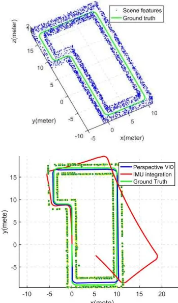
The aim of this simulation is to evaluate the performance of visual-inertial odometry with perfect visual observations. In this simulation, a total of 3000 features were randomly generated on the walls of a corridor along a ground truth trajectory with an approximate length of 77 meters. The image measurements of the features were recorded at 1Hz simulating a perspective camera moving at a constant velocity. The IMU measurements were simulated at 100 Hz using points on the ground truth trajectory. The IMU measurements were added with a constant error and a random noise for simulating the biases associated with the inertial measurements. Figure 3 shows the simulated environment with the generated feature points, the ground truth trajectory, the trajectory obtained from the simulated IMU measurements only, and the trajectory estimated by the VIO approach. It is evident that while the IMU trajectory quickly drifts away, the VIO trajectory closely follows the ground truth.
Figure 4 shows the cumulative distribution of translational and rotational errors for the perspective VIO approach and for the IMU integration. The total RMSE, defined as the root mean square of RMSEs along the trajectory, for translation and rotation are about 0.5 m and 0.04 rad respectively for the VIO approach, whereas these values for the IMU-only integration are 6.15 m and 0.24 rad. Considering the trajectory length, the perspective VIO reaches an overall positioning accuracy of 0.6% of the trajectory length compared to 8% for the IMU-only integration. Note that this accuracy is achieved without considering any feature tracking error.
Figure 3. Top: The simulated indoor environment with the generated feature points. Bottom: The top view of the simulated indoor environment and the estimated trajectory (blue) compared with the IMU trajectory (red) and the ground truth (green).
Figure 4. Left: Cumulative distribution of translational error for the perspective VIO approach and the IMU integration. Right: Cumulative distribution of rotational error for the perspective VIO approach and IMU integration.
4.2 Simulation in a photorealistic synthetic environment To study the effect of feature tracking error on the position estimation and also to evaluate the proposed OVIO, an experiment was conducted in a synthetic indoor environment created in Blender1. We generated photorealistic synthetic images for a perspective and a fisheye camera along a ground truth trajectory. To render the perspective images, we used the built-in perspective module in Blender, and for the omnidirectional images we applied an open-source patch (Zhang, et al., 2016) which is based on the Scarramuzza’s model (Scaramuzza, 2006). To simulate further research in vision-based indoor positioning, we publicly release our dataset consisting of synthetic images rendered with the perspective and fisheye cameras2. The images were recorded at 30 Hz with the resolution of 640×480 looking in the forward direction. The FoV considered for the perspective is 90º and for the fisheye is 180º. Figure 5 shows sample images of these datasets.
Figure 5. Example images from the sequence recorded using a simulated perspective camera (top) and a simulated fisheye camera (bottom).
We extracted features using the Speeded Up Robust Features (SURF) (Bay, et al., 2008) and tracked them using Kanade-Lucas-Tomasi (KLT) tracking (Tomasi & Kanade, 1991). The miss-matched points were identified as outliers and rejected by an M-estimator SAmple Consensus (MSAC) (Torr & Zisserman, 1998) algorithm with a 3-point affine transform.
1
https://www.blender.org/ 2
https://www.researchgate.net/profile/Milad_Ramezani/contributions
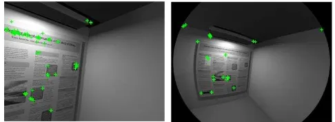
Figure 6 shows an example of feature matching results in both the perspective and the fisheye view.
Figure 6. Features after tracking process in perspective view (left) and fisheye view (right). The green pluses show the features tracked along the image sequence.
Figure 7 (left) shows a boxplot of the number of tracked features in each frame for both the perspective view and the fisheye view. The total number of tracked features in the perspective view is 1628, and in the fisheye view is 1690. Moreover, the minimum number of tracked features in the fisheye view is 17, while this value is 3 for the perspective view. Overall, the number of features tracked in the fisheye image sequence is only slightly higher than that in the perspective one. However, as it can be seen from Figure 6, the features tracked in the fisheye view cover a larger area around the camera than the perspective one, providing a better geometry for position estimation.
Figure 7. Left: Boxplot of the number of tracked features in each frame for both perspective and fisheye views. Right: Boxplot of the number of frames from which each feature is observed.
Figure 7 (right) shows a boxplot of the number of frames from which each feature is observed. The larger values for the third quartile and the maximum indicate that some features are seen over a longer sequence of images in the fisheye view than in the perspective view.
To generate the IMU measurements, we used the ground truth comprising the 3D position and 4D quaternion resampled at 300 Hz. Similar to the previous experiment, we added a constant error and a normalized random noise to simulate the static and dynamic bias of the accelerometers and gyroscopes.
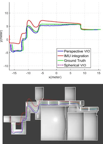
The top view of the estimated trajectories compared to the ground truth is shown in Figure 8. It can be seen that the trajectories estimated by the omnidirectional VIO and the perspective VIO closely follow the ground truth whereas the IMU trajectory exhibits a significant drift. Figure 9 shows the cumulative distribution of the translation errors and the rotation ISPRS Annals of the Photogrammetry, Remote Sensing and Spatial Information Sciences, Volume IV-2/W4, 2017
errors for the perspective and the omnidirectional VIO as well as the IMU-only integration. Clearly, the omnidirectional VIO outperforms the perspective VIO and results in more accurate position estimates. The difference in the performance of VIO and OVIO is more significant in terms of rotational accuracy, where OVIO gives rotation estimates that are 3 to 4 times more accurate than those obtained by VIO. The total length of the trajectory that the camera travelled is about 47 meters. Considering the length of the trajectory and the total error for translation, the drifts for the IMU integration, perspective and omnidirectional VIO are 9%, 1.3% and 1.1% respectively.
By comparing these results with those of the first experiment with error-free features, we can see that although the drift of the IMU integration is similar in the two experiments, the drift of the perspective VIO is approximately twice as large in the second experiment with synthetic images. This indicates that the IMU errors and the feature tracking errors contribute equally to the drift of the trajectory estimated by the visual-inertial odometry method.
Figure 8. Top view of the estimated trajectory for perspective VIO (blue), and spherical VIO (magenta) compared with the IMU only integration (red) and the ground truth (green).
Figure 9. Left: Cumulative distribution of translational error for the perspective VIO, the omnidirectional VIO and the IMU integration. Right: Cumulative distribution of rotational error
for the perspective VIO, the omnidirectional VIO and the IMU integration.
5. CONCLUSION
In this paper, we evaluated the performance of visual-inertial odometry in 3D indoor positioning. We proposed a measurement model to integrate visual observations from an omnidirectional camera with inertial measurements within a MSCKF estimation process. The results of the experiments with synthetic images of an indoor environment showed that the proposed omnidirectional visual-inertial odometry (OVIO) method outperforms the perspective VIO, and achieves a positioning accuracy of 1.1% of the length of the trajectory.
In the future, we will focus on integrating information from a Building Information Model (BIM) with the OVIO to eliminate the drift and maintain the positioning accuracy for longer distances.
ACKNOWLEDGEMENT
This work is supported by a Research Engagement Grant from the Melbourne School of Engineering, Melbourne Research Scholarship, and the China Scholarship Council - University of Melbourne Research Scholarship (Grant No. CSC 201408420117).
REFERENCES
Barreto, J. P. & Araujo, H., 2001. Issues on the geometry of central catadioptric image formation. Computer Vision and Pattern Recognition, 2001. CVPR 2001. Proceedings of the 2001 IEEE Computer Society Conference on, Kauai, Hawaii, USA, Volume 2, pp. II-II.
Bay, H., Ess, A., Tuytelaars, T. & Gool, L. V., 2008. Speeded-up robust features (SURF). Computer vision and image understanding, 110(3), pp. 346-359.
Bonin-Font, F., Ortiz, A. & Oliver, G., 2008. Visual navigation for mobile robots: A survey. Journal of intelligent and robotic systems, 53(3), p. 263.
Caruso, D., Engel, J. & Cremers, D., 2015. Large-scale direct slam for omnidirectional cameras. Intelligent Robots and Systems (IROS), 2015 IEEE/RSJ International Conference on. Hamburg, Germany, pp. 141-148.
Diel, D. D., DeBitetto, P. & Teller, S., 2005. Epipolar constraints for vision-aided inertial navigation.
Application of Computer Vision,
2005,WACV/MOTION'05, Volume 1, Seventh IEEE Workshops on, Vol 2, pp. 221-228.
Förstner, W., 2012. Minimal representations for testing and estimation in projective spaces. Photogrammetrie-Fernerkundung-Geoinformation, no. 3, pp. 209-220.
Groves, P. D., 2013. Principles of GNSS, inertial, and multisensor integrated navigation systems, Artech house, pp. 163-216.
Gu, F., Kealy, A., Khoshelham, K. & Shang, J., 2016a. Efficient and accurate indoor localization using landmark graphs. The International Archives of the Photogrammetry, Remote Sensing and Spatial Information Sciences, XLI-B2, Prague, Czech Republic ,pp. 509-514.
Gu, F., Khoshelham, K., Shang, J. & Yu, F., 2016b. Sensory landmarks for indoor localization. In Ubiquitous ISPRS Annals of the Photogrammetry, Remote Sensing and Spatial Information Sciences, Volume IV-2/W4, 2017
Positioning, Indoor Navigation and Location Based Services (UPINLBS), 2016 Fourth International Conference on, Shanghai, China, pp. 201-206.
Gu, Y., Lo, A. & Niemegeers, I., 2009. A survey of indoor positioning systems for wireless personal networks. IEEE Communications surveys & tutorials, 11(1), pp. 13-32.
Huster, A., Frew, E. W. & Rock, S. M., 2002. Relative position estimation for AUVs by fusing bearing and inertial rate sensor measurements. OCEANS'02 MTS/IEEE, Volume 3, pp. 1863-1870.
Kim, J. & Sukkarieh, S., 2007. Real-time implementation of airborne inertial-SLAM. Robotics and Autonomous Systems, 55(1), pp. 62-71.
Konstantinidis, A. et al., 2015. Privacy-preserving indoor localization on smartphones. IEEE Transactions on Knowledge and Data Engineering, 27(11), pp. 3042-3055.
Langelaan, J. W., 2007. State estimation for autonomous flight in cluttered environments. Journal of guidance, control, and dynamics, 30(5), pp. 1414-1426.
Li, M. & Mourikis, A. I., 2013. High-precision, consistent EKF-based visual-inertial odometry. The International Journal of Robotics Research, 32(6), pp. 690-711.
Liu, H., Darabi, H., Banerjee, P. & Liu, J., 2007. Survey of wireless indoor positioning techniques and systems. IEEE Transactions on Systems, Man, and Cybernetics, Part C (Applications and Reviews), 37(6), pp. 1067-1080.
Mourikis, A. I. & Roumeliotis, S. I., 2006. A Multi-State Constraint Kalman Filter for Vision-aided Inertial Navigation, Dept. of Computer Science and Engineering, University of Minnesota.
Mourikis, A. I. & Roumeliotis, S. I., 2007. A multi-state constraint Kalman filter for vision-aided inertial navigation. Robotics and automation, 2007 IEEE international conference on, Roma, Italy, pp. 3565-3572.
Nistér, D., Naroditsky, O. & Bergen, J., 2004. Visual odometry. Computer Vision and Pattern Recognition, 2004. CVPR 2004. Proceedings of the 2004 IEEE Computer Society Conference on, Washington, DC, USA, Volume 1, p. 1.
Nistér, D., Naroditsky, O. & Bergen, J., 2006. Visual odometry for ground vehicle applications. Journal of Field Robotics, 23(1), pp. 3-20.
Ong, L. L. et al., 2003. Six dof decentralised slam. Australasian Conference on Robotics and Automation, Brisbane, Australia, pp. 10-16.
Roumeliotis, S. I., Johnson, A. E. & Montgomery, J. F., 2002. Augmenting inertial navigation with image-based motion estimation. Robotics and Automation, 2002. Proceedings. ICRA'02. IEEE International Conference on, Washington, D.C., USA, Volume 4, pp. 4326-4333.
Scaramuzza, D. A. M. a. R. S., 2006. A flexible technique for accurate omnidirectional camera calibration and structure from motion. Computer Vision Systems, 2006 ICVS'06. IEEE International Conference on, New York, USA, pp. 45-45.
Tomasi, C. & Kanade, T., 1991. Detection and tracking of point features.
Torr, P. & Zisserman, A., 1998. Robust computation and parametrization of multiple view relations. Computer
Vision, 1998. Sixth International Conference on, Bombay, India, pp. 727-732.
You, S. & Neumann, U., 2001. Fusion of vision and gyro tracking for robust augmented reality registration. Virtual Reality, 2001. Proceedings. IEEE, Yokohama, Japan, pp. 71-78.
Zhang, Z., Rebecq, H., Forster, C. & Scaramuzza, D., 2016. Benefit of large field-of-view cameras for visual odometry. In Robotics and Automation (ICRA), 2016 IEEE International Conference on, Stockholm, Sweden, pp. 801-808.