SEGMENTATION OF ENVIRONMENTAL TIME LAPSE IMAGE SEQUENCES FOR
THE DETERMINATION OF SHORE LINES CAPTURED BY HAND-HELD
SMARTPHONE CAMERAS
M. Kröhnerta, *, R. Meichsner a
a Technische Universität Dresden, Institute of Photogrammetry and Remote Sensing, 01069 Dresden - (melanie.kroehnert, robert.meichsner)@tu-dresden.de
Commission IV, WG IV/4
KEY WORDS: Flood monitoring, Geo-crowdsourcing, Spatio-temporal texture, Time lapse image analysis, Smartphone application
ABSTRACT:
The relevance of globally environmental issues gains importance since the last years with still rising trends. Especially disastrous floods may cause in serious damage within very short times. Although conventional gauging stations provide reliable information about prevailing water levels, they are highly cost-intensive and thus just sparsely installed. Smartphones with inbuilt cameras, powerful processing units and low-cost positioning systems seem to be very suitable wide-spread measurement devices that could be used for geo-crowdsourcing purposes. Thus, we aim for the development of a versatile mobile water level measurement system to establish a densified hydrological network of water levels with high spatial and temporal resolution. This paper addresses a key issue of the entire system: the detection of running water shore lines in smartphone images. Flowing water never appears equally in close-range images even if the extrinsics remain unchanged. Its non-rigid behavior impedes the use of good practices for image segmentation as a prerequisite for water line detection. Consequently, we use a hand-held time lapse image sequence instead of a single image that provides the time component to determine a spatio-temporal texture image. Using a region growing concept, the texture is analyzed for immutable shore and dynamic water areas. Finally, the prevalent shore line is examined by the resultant shapes. For method validation, various study areas are observed from several distances covering urban and rural flowing waters with different characteristics. Future work provides a transformation of the water line into object space by image-to-geometry intersection.
1. INTRODUCTION
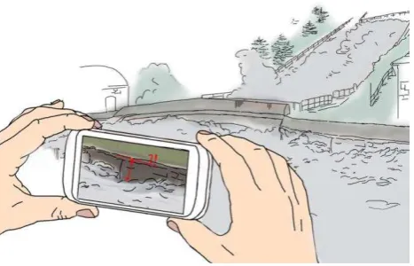
Because of huge costs, the overall observation of flood-prone areas by permanently installed measurement stations is often just scantily available. Unfortunately, several hydrological networks have an insufficient coverage for the effected regions of interest (ROI) in case of need. Minor rivers are often neglected but ensure serious damages in case of flash floods. A small municipality called Braunsbach in Baden-Wuerttemberg, Germany received worldwide recognition in summer of 2016. After heavy rainfalls, a small river passing Braunsbach became a devastating stream with high increased flow rates by more than 500 times compared to flood situations known there. Exact values are not available due to only one measurement station, located approximately 10 km away from the hot spots. High waters and several landslides led to high structural damages and complicated rescue operations (Agarwal et al., 2016). For the development of a versatile mobile water level measurement system, the necessary input data is provided by geo-crowdsourcing using smartphones to capture and process hand-held time lapse image sequences to extract the prevalent water line as a basic requirement for the observation of water level changes (see Figure 1). Subsequently, the detected water line has to be transferred into object space to determine the final water level (not addressed in this paper). However, the segmentation of running water and nearshore environment is a non-trivial task and has been treated frequently in image processing fields (see Section 1.1). An individual image is only a snapshot which barely covers the characteristics of non-rigid objects like water. In addition to the image space, the use of the time axis provides an efficient complement for image segmentation by means of spatio-temporal variability.
* Corresponding author
Figure 1. Schematic use case of water level determination using hand-held smartphone.
respectively the predominant dynamic or static part of the ROI and must be analyzed for their spatio-temporal distribution to assess the texture significance (see Section 3.3). Depending on the results, an automatic steered region growing is applied for image segmentation (see Section 3.4). Using the specified regions, the prevalent shore line is investigated and described in Section 3.5. Whereas Section 4 illustrates the resulting water lines of the introduced study areas, Section 5 gives an evaluation respectively. The paper ends with a critical examination of the proceeding and give a short outlook for future work (see Section 6).
1.1 Related work
In geosciences, especially in remote sensing, multispectral imagers provide spectral signatures from natural objects depending on their physical conditions, like the approved NDWI for water recognition (Feyisa et al., 2014; Gao, 1996; Li et al., 2014; Sarp and Ozcelik, 2016). Currently, it seems to be obvious that the application of mobile multispectral imaging using smartphones is not possible due to technical reasons.
An alternative approach is provided by the analysis of image texture. A fundamental work written by Haralick et al. (1973), defines texture as ‘one of the important characteristics used in identifying objects of regions of interests in an image, whether the image be a photomicrograph, an aerial photograph, or a satellite image’. Thus, the combined application of single textural features and spectral information has been proven for image classification and was frequently applied and enhanced for precise image segmentation in geosciences (Kim et al., 2009; Ferro and Warner, 2002; Martino et al., 2003; Verma, 2011; Zhang, 1999). But, the calculation of various texture features requires high performance which may impede the use of smartphones beside flagship systems. Referring to Varma and Zisserman (2005), ‘a texture image is primarily a function of the following variables: the texture surface, its albedo, the illumination, the camera and its viewing position. Even if we were to keep the first two parameters fixed, i.e. photograph exactly the same patch of texture every time, minor changes in the other parameters can lead to dramatic changes in the resultant image. This causes a large variability in the imaged appearance of a texture and dealing with it successfully is one of the main tasks of any classification algorithm.’ In contrast to remote sensing, texture surfaces of close-range camera observations are highly affected by the mentioned influence factors regarding varying camera constellations. Tuceryan and Jain (1993) termed texture as a ‘prevalent property of most physical surfaces in the natural world’ which is why motion has to be treated as textural criterion as well. Figure 2 demonstrates the strongly different appearances of running waters due to varying camera constellations and mutable image content. The complementary use of time and space enables the investigation of spatio-temporal texture and thus a situation-based image segmentation in respect of time-dependent image content (Szummer and Picard, 1996; Peh and Cheong, 2002; Hu et al., 2006; Nelson and Polana, 1992; Xu et al., 2011). On this basis, we add the temporal variability by means of time lapse image sequences. Subsequently, the proper segmentation starts in accordance to the defined feature space. Several approaches prefer a supervised classification that may be enhanced by deep neural networks for training robust classifiers (Maggiori et al., 2017; He et al., 2016; Ciregan et al., 2012; Krizhevsky et al., 2012; Reyes-Aldasoro and Aldeco, 2000). Moreover, the investigation of a sufficient training dataset for image classification regarding running waters, appears rather difficult. In conclusion, the presented approach for water line
detection is primarily based on image segmentation and classification which must fulfil two basic criteria: firstly, the algorithm deals with running waters high variability and secondly, it should be appropriate to run on common smartphone devices. Thus, high intensive processing should be avoided as much as possible.
Figure 2. Appearances of different running waters, captured with varying camera constellations.
A similar approach provided by Kröhnert (2016), successfully demonstrates the segmentation of running water and shore land using spatio-temporal texture. However, the approach has issues regarding rotation invariance of the water line location within the image and processing time. Besides this, the implemented segmentation uses hard-defined parameters which may fail in cases of running waters with highly different characteristics than the presented one. Our approach enhances the calculation of spatio-temporal texture regarding processing time and demonstrates an orientation-invariant segmentation procedure due to multiple seeded region growing (see Section 3.4) with automatic set up avoiding empirical determined parameters (see Section 3.2).
2. DATA
Considering variable image content of close-range images, the texture of an individual image will not have a generally valid significance for proper image segmentation which is why our approach regards the time component. By means of time lapse image sequences, the mutable textures provide significant advantages for image classification (e.g. reflections on running water surfaces). Moreover, it allows for image segmentation and thus for boundary extraction like shore lines by means of the mapped dynamics only.
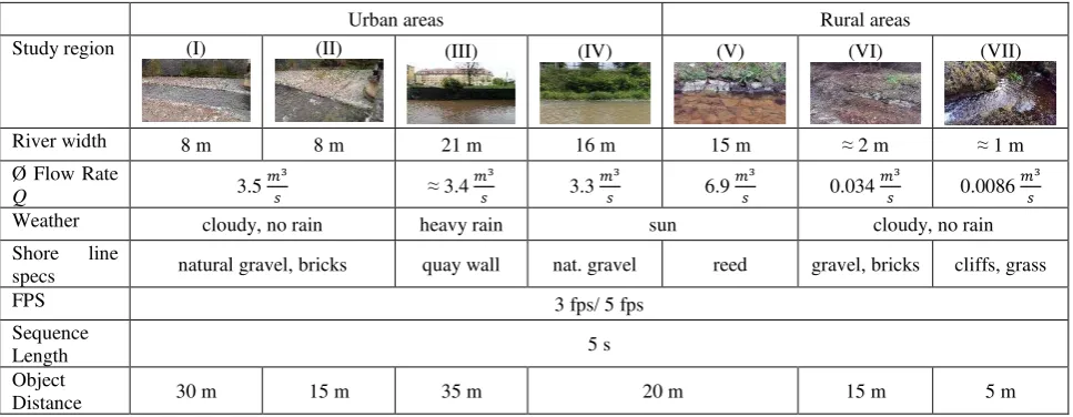
Table 1. Study areas covering urban and rural running waters regarding situative specifications of environment and camera configurations.
The urban scenes correspond to one river with different forms of appearance and characteristics due to varying points of view and camera distances. For the investigation of rural waters, we have observed two small creeks and one large river in forest areas using a HTC One M7 smartphone, released in 2013, as measurement device with operating system Android 5.1. Thereby, the dimension of the time lapse image sequences amounts to 1920 x 1080 pixels in all test cases. Furthermore, the temporal variability is easily assessable though the number of images within the time lapse image sequence. Thus, two combinations of frame rate and sequence length are investigated in order to test the dependency of flow velocity and time lapse. Table 1 gives a detailed overview over the investigated areas and environmental conditions for image capturing.
3. APPLICATION DEVELOPMENT
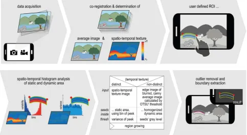
The process pipeline, illustrated in Figure 3, starts with the preliminary work of time lapse image sequence co-registration in direct succession to the initially data acquisition. By means of the gray level magnitudes concerning the co-registered image sequence (see Section 3.1), the corresponding spatio-temporal texture as well as the mean value (hereinafter referred to as ’average image’) will be calculated pixel by pixel (see Section 3.2). Afterwards, human interaction takes place in the form of a coarse selection of the shore line to be extracted. For this, a graphical user interface (GUI) is used displaying the calculated average image to the user, which depicts a virtually homogenized surface of the dynamic image part (see Figure 3, top right).
The resultant image areas mark either the predominant dynamic or static part of the ROI. Both regions are analyzed for their spatio-temporal distribution to assess the prevalent texture significance (see Section 3.3). Possibly for slow-running rivers or large object distances, the spatio-temporal texture may not have sufficient resolution to serve as appropriate input for image segmentation purposes. In this case, the average image of the time lapse sequence provides a basis for the further processing.
The segmentation process itself (see Section 3.4) is automatic steered and demands an automatic definition of input data and variables. The data required for this purpose bases on the results of the previously texture significance analyses. For both options,
Section 3.4.1 and Section 3.4.2 describe the automatic definition of variables, necessary for the following segmentation with the application of region growing (see Section 3.4). Finally, the resultant image segments are analyzed for the prevalent shore line (see Section 3.5).
3.1 Time lapse image sequence co-registration
After image acquisition, an attempt is being made to co-register all individual images of a time lapse image sequence. In doing so, the first scene acts as so-called master image whereas all remaining images will be treated as slaves. In principle, we calculate the image homographies respectively for all slave images in dependence on the master scene. Consequently, all co-registered images belong to the geometry of the master image. The procedure comprises in general the repeated detection and description of potential key points, their matching and finally the homography calculation using suitable matches to carry out the perspective transformation. For the App implementation, we make use of OpenCV’s framework, version 3.1.0 for Android development (Bradski, 2000).
Using the Harris-Operator presented by Harris and Stephens (1988) for the fast detection of potential feature points in each image, only image points that refer to discrete corners are considered like stones, railings or walls. For feature description, we use the scale-invariant feature transform (SIFT) algorithm followed by fast feature point matching, described in Lowe (2004) and Muja and Lowe (2009). At least we need a minimum of four good matches to calculate the homography of each master-slave image pair. Otherwise, the slave has to be rejected (which may result due to blurred images). In doing so, RANSAC is applied with a threshold of three pixels to detect and eliminate outliers affecting the transformation. With the aid of the estimated slave image points that refer to individual positions as a function of the master point coordinates, the slave images could be co-registered in consideration of the master geometry using a perspective transformation with cubic interpolation. Obviously, the approach does not need further input data for image registration, but account must be taken during data acquisition. The homographies may not handle major changes in scale well which means that the camera must be held steadily until the acquisition has finished. However, this should not cause problems in case of short time
specs natural gravel, bricks quay wall nat. gravel reed gravel, bricks cliffs, grass
FPS 3 fps/ 5 fps
Sequence
Length 5 s
Object
Figure 3. Process pipeline from data acquisition to result display.
3.2 Investigation of spatio-temporal texture
The investigation of spatio-temporal texture as well as the average image are treated relating to previously introduced image co-registration. Moreover, the transformed images are checked in a consecutive manner for absolute pixel differences. Difference images thus generated are summed up and map the magnitude of spatio-temporal variability known as spatiotemporal texture (see Figure 3, bottom). Additionally, the average image of the processed image sequence is calculated pixel by pixel per mean value. Referring to this, the appearance of the original dynamic image content belongs to a homogenized surface, depending on image frequency and observation time. In case of time lapse sequences, the representation of running rivers looks almost homogeneous or smoothed. Figure 4 shows a single image of a shallow urban river (study area (I)) in comparison to its average image and the appropriate spatio-temporal texture, calculated with 15 co-registered images (3 fps, 5 s).
3.3 Histogram analysis
After texture calculation, the user is requested to trace the water line within the displayed average image (see Figure 3, top right). In doing so, every selected image point that refers to the initial water line is captured. To specify the ROI for further processing, the line has to be expanded by a defined value orthogonally using the respective points. The extension value initially amounts to 50 pixels but can be adapted using the GUI to fit the prevalent camera resolution and object distance. Using the water line selection and the buffered region, one of the halves represents the major part of static and the other one the part of dynamic features. Closing up, the algorithm is trained by a single finger tap inside the most static image region which refers to the land area.
Immediately afterwards, the temporal variability of both regions is investigated respectively through spatio-temporal histograms (see Figure 3, bottom left). The number of bins amounts to the
spatiotemporal magnitudes within the defined ROI. We assume that both histograms are highly different because of immutable and non-rigid image contents. Afterwards, both histograms are correlated to qualify their similarity. In case of a correlation coefficient less than 90 %, both regions can be clearly separated by pixels spatio-temporal variability. Consequently, the spatiotemporal texture provides a sufficient basis for the segmentation via the characteristics of imaged dynamics.
Figure 4. Detail view of a co-registered time lapse image sequence taken with 3 fps over 5 s in study area (I). Top down:
master image, associated average image & spatio-temporal texture visualized by observed pixel magnitudes ���.
However, less spatiotemporal texture is associated with less variabilities inside of the imaged running water. Thus, average image serves as a complementary alternative for the following segmentation of water and environment due to its homogeneous appearance. Both types are visualized in Figure 5 and Figure 6.
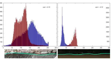
Figure 5. Histogram analyses of spatio-temporal textures in relation to respective ROIs. Left: Study area (II), dissimilarities
enable spatio-temporal texture, correlation factor corr = 0.08. Right: less spatio-temporal variability (corr = 0.97).
Figure 6. Histogram analysis of average image in respect of respective ROIs. Left: gray level distribution of mean values provides no useful information for image segmentation. Right: Study area (III), classifiable due to homogenized image content
by averaged gray values.
For shallow water in study area (I) it could be noticed that the spatio-temporal texture provides a good basis for image segmentation with respect to the static area. In contrast to this, the average image holds good for a region growing-based image separation in consideration of the homogenized water surface, approved in study area (III).
3.4 Image segmentation by region growing
Depending on the results of the histogram analysis, either the spatio-temporal texture or the average image serves as input for image segmentation. We decided to use region growing because of its simplicity due to multiple seed point definition with a clear representation of image properties as well as its robustness against image noise (Kamdi and Krishna, 2012). Moreover, region growing is able to detect connected regions in dependency of variable pixel neighborhoods. A well-known shortcoming of region growing is the high computation time. Hence, we use the defined ROI to restrict the search area which enhances the processing time significantly.
The approach compares the prevalent attributes of a seed point with the characteristics of its close proximity. In doing so, a defined threshold value (or vector for multiple attributes) serves as a criterion for similarity between the starting point and the investigated neighborhood. If similarity is given, the considered
points belong to one image segment whose boundary provides the points now to check for neighbor affiliations. In case of non-fitting points or when the boundary of the defined ROI is reached, the procedure terminates.
According to the input data the parameters for both, seed point and threshold should be defined automatically. Section 3.4.1 describes the steering based on the spatio-temporal texture whereas Section 3.4.2 regards the approach using the average image.
3.4.1 Segmentation by spatio-temporal texture analysis: In case of significant spatio-temporal texture, the definition of seed points depends on the initial masked area that relates primarily to immutable image content. Probably, changes which may occur from weather influences like rainfall or changing light conditions in case of moving clouds would lead to spatio-temporal noise. Another reason for noise may cause by small residual errors in the image sequence co-registration. Thus, we look for a threshold that corresponds to the main area of static image content while neglecting outliers. A solution for the issue is provided by the associated histogram whereas the threshold belongs to the most prevalent magnitude. Image points whose attributes equals the threshold value are carried out as potential seed points. One of the seeds is randomly selected as starting point for a first iteration. All values that show less or equal temporal stability � , ≤
ℎ � ℎ are assigned to the region of immutable image content.
The remaining seeds are checked for their region assignment and if necessary, the process repeats until all predefined seeds are in connection by means of the developed region. This conversely means that the left pixels within the ROI point to dynamic image content and thus to running water (see Figure 7).
Figure 7. Spatio-temporal texture overlay referring to study region (II). White polygon: ROI from coarse water line preselection, Blue polygon: Initial water body pointing to
dynamic image content; Red dots: Potential seed points.
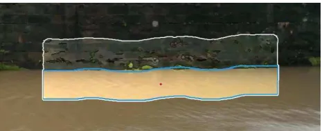
Figure 8. Average image with canny edge map overlay of study region (III); White polygon: ROI from coarse water line preselection; Blue polygon: Initial water body pointing to
homogenized dynamic image content; Red: Seed point.
3.5 Water line detection
Closing the processing, the water line is derived using the observed image segments. Whether for the region of immutable image content, examined by spatio-temporal texture or for the Growing can detect undercuts which may occur e.g. due to rising stones in the near shore area. For our water level monitoring system, we only need one shoreline which is why we eliminate such occurrences by means of Cleveland’s Locally Weighted Regression (Cleveland, 1979).
4. EXPERIMENTAL RESEARCH AND RESULTS
As already was mentioned, we apply the algorithm in different study areas using several camera constellations and two time lapse configurations respectively (see Table 1 above). Regarding each processing step, the processing times are listed in Table 2. The size of bounding boxes (labeled ’BBox’ in Table 2) helps to qualify the processing time regarding the initial ROI. It should be mentioned that the first step refers to the whole image to ensure a sufficient number of suitable features for image co-registration regarding the running water environment. Both, the average and the spatio-temporal texture are generated parallel to the images co-registration but without a significant influence to processing time. The investigation results for the urban study areas (I)-(IV) and the rural areas (V)-(VII) are visualized in detail in Table 3 (description in caption).
5. EVALUATION AND DISCUSSION
Our paper presents a reliable approach for mobile image segmentation on the basis of mapped image dynamics with the objective of a versatile water level measurement system. We show an enhancement of the approach from Kröhnert (2016) with respect to processing time and image adjustment, proven in several urban and rural regions with differing running rivers and environmental situations. Furthermore, we integrate an alternative processing for images with less spatio-temporal information. Our approach is (semi-) automatically steered with a unique user interaction to define the region of interest.
As being expected, the bottleneck regarding processing times occurs due to images co-registration. The longest times are taken by feature detection and description using SIFT that affects the first processing step only in respect of varying frame rates. The times for the remaining processing steps stay -compared to the different frame rates- mostly the same or very close together
which is why we have not provided an individual statement for each (see Table 2). Compared to other feature detectors like ORB (see Kröhnert, 2016), SIFT’s accuracy and robustness were given priority over processing time. Naturally, the hard tasks are processed in background to avoid an overloaded UI thread.
In conclusion, the water line could be successfully derived in all experiments. Thereby, a time lapse initialization with a frame rate of 3 fps and a sequence length of 5 s seems to be the best combination that covers the most urban and land river characteristics due to flow velocity and does take account of processing time. Higher frame rates result in more images being processed and thus to avoidable long processing times. Furthermore, Table 2 shows that the processing time increases nearly exponential with respect of the image number. In this connection, an important point that should be kept in mind is the spatio-temporal noise which may occur due to scaling issues during homography calculations. The stronger users motion and the higher the number of images, the more noise may occur and distort the result (see Table 3, study area (V)). The same applies for high changing backgrounds of shore environments which may lead to a high amount of falsely taken key points that could not be detected by RANSAC (e.g. vegetation moving in the wind).
Finally, it should be noticed that the investigated boundary reflects the mapped situation and is valid for the corresponding observation time only. For the derivation of instantaneous water levels, this may not be relevant but should be considered in relation to other possible applications.
6. FUTURE WORK
To improve the approach, future enhancements could deal with the bottleneck of processing time by outsourcing calculations to the graphic chip (GPU processing). Furthermore, the region growing needs more investigation in case of occurring leaks that are a frequently treated problem in image processing concerning region growing approaches. In our investigations, we have not detected large leaks but we cannot exclude that they will not have influences on water line derivation in general.
The main aspect being developed comprises the intersection of the derived water line and digital terrain data to transfer the image to the object space which allows for the on-the-fly water level determination. Moreover, we will be able to verify the derived water levels with conventionally acquired data and estimate the accuracy.
ACKNOLODGEMENTS
Gratefully, we acknowledge the European Social Fund (ESF) and the Free State of Saxony for their financial support on a grant.
REFERENCES
Agarwal, A., Boessenkool, B., Fischer, M. and other, 2016. Die Sturzflut in Braunsbach, Mai 2016. Eine Bestandsaufnahme und Ereignisbeschreibung. Final Report Taskforce DFG graduate college Natural Hazards and Risks in a Changing World: ‘Flash Flood in Braunsbach (Germany) in May 2016’.
Bradski, G., 2000. The opencv library. Dr. Dobb’s Journal of Software Tools.
Canny, J., 1986. A computational approach to edge detection.
IEEE Transactions on pattern analysis and machine intelligence
Ciregan, D., Meier, U. and Schmidhuber, J., 2012. Multi-column deep neural networks for image classification. In: IEEE Conference on Computer Vision and Pattern Recognition (CVPR), 2012, IEEE, pp. 3642–3649.
Cleveland, W. S., 1979. Robust locally weighted regression and smoothing scatterplots. Journal of the American statistical association 74(368), pp. 829–836.
Fang, M., Yue, G. and Yu, Q., 2009. The study on an application of otsu method in canny operator. In: International Symposium on Information Processing (ISIP), Citeseer, pp. 109–112.
Ferro, C. J. S. andWarner, T. A., 2002. Scale and texture in digital lmage classification. Photogrammetric Engineering & Remote Sensing 68(1), pp. 51–63.
Feyisa, G. L., Meilby, H., Fensholt, R. and Proud, S. R., 2014. Automated water extraction index: A new technique for surface water mapping using landsat imagery. Remote Sensing of Environment 140, pp. 23–35.
Gao, B.-C., 1996. Ndwia normalized difference water index for remote sensing of vegetation liquid water from space. Remote sensing of environment 58(3), pp. 257–266.
Haralick, R. M., Shanmugam, K. and Dinstein, I. H., 1973. Textural features for image classification. IEEE Transactions on Systems, Man and Cybernetics 6, pp. 610–621.
Harris, C. and Stephens, M., 1988. A combined corner and edge detector. In: Alvey vision conference 15, Citeseer, p. 50.
He, K., Zhang, X., Ren, S. and Sun, J., 2016. Deep residual learning for image recognition. In: The IEEE Conference on ComputerVision and Pattern Recognition (CVPR).
Hu, Y., Carmona, J. and Murphy, R. F., 2006. Application of temporal texture features to automated analysis of protein subcellular locations in time series fluorescence microscope images. In: 3rd IEEE International Symposium on Biomedical Imaging: Nano to Macro, 2006, IEEE, pp. 1028–1031.
Kamdi, S. and Krishna, R. K., 2012. Image segmentation and region growing algorithm. In: International Journal of Computer Technology and Electronics Engineering (IJCTEE) 2.
Kim, M., Madden, M. and Warner, T. A., 2009. Forest type mapping using object-specific texture measures from multispectral ikonos imagery. Photogrammetric Engineering & Remote Sensing 75(7), pp. 819–829.
Koschitzki, R., Schwalbe, E. and Maas, H.-G., 2014. An autonomous image based approach for detecting glacial lake outburst floods. The International Archives of Photogrammetry, Remote Sensing and Spatial Information Sciences 40(5), pp. 337.
Krizhevsky, A., Sutskever, I. and Hinton, G. E., 2012. Imagenet classification with deep convolutional neural networks. In:
Advances in neural information processing systems, pp. 1097–
1105.
Kröhnert, M., 2016. Automatic waterline extraction from smartphone images. The International Archives of the Photogrammetry, Remote Sensing and Spatial Information Sciences 41(5), pp. 857–863.
Li, B., Zhang, H. and Xu, F., 2014. Water extraction in high resolution remote sensing image based on hierarchical spectrum
and shape features. In: IOP Conference Series: Earth and Environmental Science 17(1), IOP Publishing, p. 012123.
Lowe, D. G., 2004. Distinctive image features from scaleinvariant keypoints. International journal of computer vision 60(2), pp. 91–110.
Maas, H.-G., Casassa, G., Schneider, D., Schwalbe, E. and Wendt, A., 2010. Photogrammetric determination of spatiotemporal velocity fields at glaciar san rafael in the northern Patagonian icefield. The Cryosphere Discussions 4(4), pp. 2415–
2432.
Maggiori, E., Tarabalka, Y., Charpiat, G. and Alliez, P., 2017. Convolutional neural networks for large-scale remote-sensing image classification. IEEE Transactions on Geoscience and Remote Sensing 55(2), pp. 645–657.
Martino, M. D., Causa, F. and Federico, S. B., 2003. Classification of optical high resolution images in urban environment using spectral and textural information. In: Proc. IGARSS 2003 1, IEEE, pp. 467–469.
Muja, M. and Lowe, D. G., 2009. Fast approximate nearest neighbors with automatic algorithm configuration. VISAPP (1)
2(331-340), pp. 2.
Nelson, R. C. and Polana, R., 1992. Qualitative recognition of motion using temporal texture. CVGIP: Image understanding
56(1), pp. 78–89.
Otsu, N., 1975. A threshold selection method from gray-level histograms. Automatica 11(285-296), pp. 23–27.
Peh, C.-H. and Cheong, L.-F., 2002. Synergizing spatial and temporal texture. IEEE Transactions on Image Processing
11(10), pp. 1179–1191.
Reyes-Aldasoro, C. C. and Aldeco, A. L., 2000. Image segmentation and compression using neural networks. In: Proc. Advances Artificial Perception Robotics, 2000.
Sarp, G. and Ozcelik, M., 2016. Water body extraction and change detection using time series: A case study of lake burdur, turkey. Journal of Taibah University for Science.
Szummer, M. and Picard, R. W., 1996. Temporal texture modeling. In: Proceedings. International Conference on Image Processing 1996, IEEE, 3 pp. 823–826.
Tuceryan, M. and Jain, A. K., 1993. Texture analysis. Handbook of pattern recognition and computer vision 2, pp. 207–248.
Varma, M. and Zisserman, A., 2005. A statistical approach to texture classification from single images. International Journal of Computer Vision 62(1-2), pp. 61–81.
Verma, A., 2011. Identification of land and water regions in a satellite image: a texture based approach. International Journal of Computer Science Engineering and Technology 1, pp. 361–
365.
Xu, Y., Quan, Y., Ling, H. and Ji, H., 2011. Dynamic texture classification using dynamic fractal analysis. In: International Conference on Computer Vision 2011, IEEE, pp. 1219–1226.
Zhang, Y., 1999. Optimisation of building detection in satellite images by combining multispectral classification and texture filtering. ISPRS Journal of Photogrammetry and Remote Sensing
Urban areas Rural areas Study region
BBox
(I) (765x140)
(II) (1395x135)
(III) (1755x185)
(IV) (550x165)
(V) (984x216)
(VI) (692x253)
(VII) (643x213) Processing times
Frame rate 3 5 3 5 3 5 3 5 3 5 3 5 3 5
Step 1 45.4 83.3 43.9 86.0 47.1 78.5 44.5 80.3 47.8 86.2 44.3 85.1 43.1 83.2
Step 2 1.4 1.9 0.8 0.6 1.0 1.4 1.2
Step 3 9.1 12.1 6.4 6.7 5.6 4.7 3.8
Step 4 0.3 0.4 0.4 0.1 0.2 0.2 0.1
Table 2. Summary of processing times regarding two frame rates of 3 & 5 fps with a time lapse interval of 5 seconds to observe the study areas (I)-(VII). Bounding box (BBox) for ROI description in pixels. Processing times in seconds with respect to single processing steps: (1) Co-registration, average image & spatio-temporal texture calculation, (2) Histogram analysis & initialization of
step (3) image segmentation, (4) water line extraction.
Investigation of urban areas
(I) (II) (III) (IV)
Investigation of rural areas
(V) (VI) (VII)
Table 3. Experimental investigations of water lines using the spatio-temporal texture (urban study areas (I) & (II)) and rural areas (V)-(VII)) or the average image (urban study areas (III) & (IV)) for image segmentation. Top rows: Overlay of average & spatio-temporal texture image containing masked ROI & initial shore line (red). Lower lines: determined water line using 3 fps (blue) &