Intra-day Trading of the FTSE-100 Futures Contract Using Neural Networks With Wavelet Encodings

Submitted to European Jo urnal of Finance

Intra-day Trading of the FTSE-100 Futures Contract

Using Neural Networks With Wavelet Encodings

D L Toulson

S P Toulson

∗

Intelligent Financial Systems Limited

Suite 4.2 Greener House

66-69 Haymarket

London SW1Y 4RF

SW1Y 4RF

Tel: (020) 7839 1863

Email:

ifs@if5.com

www.if5.com

Intra-day Trading of the FTSE-100 Futures Contract

Using Neural Networks With Wavelet Encodings

ABSTRACT

In this paper, we shall examine the combined use of the Discrete Wavelet Transform and regularised neural networks to predict intra-day returns of the FTSE-100 index future. The Discrete Wavelet Transform (DWT) has recently been used extensively in a number of signal processing applications. The manner in which the DWT is most often applied to classification / regression problems is as a pre-processing step, transforming the original signal to a (hopefully) more compact and meaningful representation. The choice of the particular basis functions (or child wavelets) to use in the transform is often based either on some pre-set sampling strategy or on a priori heuristics about the scale and position of the information likely to be most relevant to the task being performed.

In this work, we propose the use of a specialised neural network architecture (WEAPON) that includes within it a layer of wavelet neurons. These wavelet neurons serve to implement an initial wavelet transformation of the input signal, which in this case, will be a set of lagged returns from the FTSE-100 future. We derive a learning rule for the WEAPON architecture that allows the dilations and positions of the wavelet nodes to be determined as part of the standard back-propagation of error algorithm. This ensures that the child wavelets used in the transform are optimal in terms of providing the best discriminatory information for the prediction task.

We then focus on additional issues re lated to use of the WEAPON architecture. First, we examine the inclusion of constraints for enforcing orthogonality in the wavelet nodes during training. We then propose a method (M&M) for pruning excess wavelet nodes and weights from the architecture during training to obtain a parsimonious final network. We will conclude by showing how the predictions obtained from committees of WEAPON networks may be exploited to establish trading rules for adopting long, short or flat positions for the FTSE-100 index future using a Signal Thresholded Trading System (STTS). The STTS operates by combining predictions of future returns over a variety of different prediction horizons. A set of trading rules is then determined that act to optimise the Sharpe Ratio of the trading strategy using realistic assumptions for bid/ask spread, slippage and transaction costs.

1

Introduction

Over the past decade, the use of neural networks for financial and econometric applications has been widely researched (Refenes et al [1993], Weigend [1996], White [1988] and others). In particular, neural networks have been applied to the task of providing forecasts for various financial markets ranging from spot currencies to equity indexes. The implied use of these forecasts is often to develop systems to provide profitable trading recommendations.

However, in practice, the success of neural network trading systems has been somewhat poor. This may be attributed to a number of factors. In particular, we can identify the following weaknesses in many approaches:

1. Data Pre-processing – Inputs to the neural network are often s imple lagged returns (or even prices!). The dimension of this input information is often much too high in the light of the number of training samples likely to be available. Techniques such as Principal Components Analysis (PCA) (Oja [1989]) and Discriminant Analysis (Fukunaga [1990]) can often help to reduce the dimension of the input data as in Toulson & Toulson (1996a) and Toulson & Toulson (1996b) (henceforth TT96a, TT96b). In this paper, we present an alternate approach using the Discrete Wavelet Transform (DWT).

2. Model Complexity – Neural networks are often trained for financial forecasting applications without suitable regularisation techniques. Techniques such as Bayesian Regularisation MacKay (1992a), MacKay (1992b) (henceforth M92a, M92b) Buntime & Weigend(1991) or simple weight decay help control the complexity of the mapping performed by the neural network and reduce the effect of over-fitting of the training data. This is particularly important in the context of financial forecasting due to the high level of noise present within the data.

3. Confusion Of Prediction And Trading Performance – Often researchers present results for financial forecasting in terms of root mean square prediction error or number of accurately forecasted turning points. Whilst these values contain useful information about the performance of the predictor they do not necessarily imply that a successful trading system may be based upon them. The performance of a trading system is usually dependent on the performance of the predic tions at key points in the time series. This performance is not usually adequately reflected in the overall performance of the predictor averaged over all points of a large testing period.

We shall present a practical trading model in this paper that attempts to address each of these points.

2

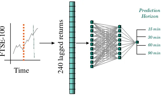
The Prediction Model

240 lagged returns

FTSE-100

Time

15 min 30 min 60 min 90 min

Prediction Horizon

Figure 1: Predicting FTSE -100 Index Futures: 240 lagged returns are extracted form the FTSE -100 future time series. These returns are used as input to (WE A PON ) ML Ps. Different ML Ps are trained to predict the return of the F TSE -100 future

15, 30, 60 and 90 minutes ahead.

A key consideration concerning this type of prediction strategy is how to encode the 240 available lagged returns as a neural network input vector. One possibility is to simply use all 240 raw inputs. The problem with this approach is the high dimensionality of the input vectors. This will require us to use an extremely large set of training examples to ensure that the parameters of the model (the weights of the neural network) may be properly determined. Due to computational complexities and the non-stationarity of financial time series, using extremely large training sets is seldom practical. A preferable strategy is to reduce the dimension of the input information to the neural network.

A popular approach to reducing the dimension of inputs to neural networks is to use a Principal Components Analysis (PCA) transform to reduce redundancy in the input vectors due to inter-component correlations. However, as we are working with lagged returns from a single financial time series we know, in advance, that there is little (auto) correlation in the lagged returns. In other work (TT96a), (TT96b), we have approached the problem of dimension reduction through the use of Discriminant Analysis techniques. These techniques were shown to lead to significantly improved performance in terms of prediction ability of the trained networks.

However, such techniques do not, in general, take any advantage of our knowledge of the temporal structure of the input components, which will be sequential lagged returns. Such techniques are also implicitly linear in their assumptions of separability, which may not be generally appropriate when considering inputs to (non-linear) neural networks.

. .

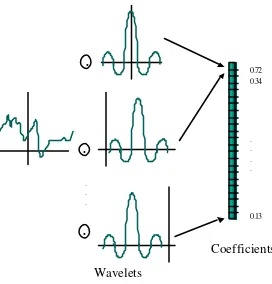
Wavelets

Coefficients

. . .

.

.

.

0.72 0.34

. . . .

0.13

Figure 2: The discrete wavelet transform. The time series is convolved with a number of child wavelets characterised by different dilations and translations of a particular mother

wavelet..

3

The Discrete Wavelet Transform (DWT)

3.1 Background

The Discrete Wavelet Transform (Telfer et al [1995], Meyer [1995]) has recently received much attention as a technique for the pre -processing of data in applications involving both the compact representation of the original data (i.e. data compression or factor analysis) or as a discriminatory basis for pattern recognition and regression problems (Casasent & Smokelin [1994], Szu & Telfer [1992]).

The transform functions by projecting the original signal onto a sub-space spanned by a set of child wavelets derived form a particular Mother wavelet.

For example, let us select the Mother wavelet to be the Mexican Hat function

( )

1

.

3

2

)

(

4 2 2

1 _t2

e

t

t

y

=

π

−

− (1)

The wavelet children of the Mexican Hat Mother are the dilated and translated forms of (1), i.e.

φ

ζ

φ

τ

ζ

τ ζ,

( )

t

=



t

−







_



1

(2)

Now, let us select a finite subset C from the infinite set of possible child wavelets. Let the members of the subset be identified by the discrete values of position

τ

_i and scale

ζ

_i,

i

=

1

,...,

K

,

{

}

C

=

τ ζ

i

,

i

i

=

1

,...,

K

(3)

Suppose we have an N dimensional discrete signal

x

ρ

. The jth component of the projection of the original signal

x

ρ

onto the

K

dimensional space spanned by the child wavelets is then

y

j

x

i

i N

i j j

=

=

∑

1

φ

τ ζ,

( )

(4)

3.2 Choice of Child Wavelets

The significant questions to be answered with respect to using t he DWT to reduce the dimension of the input vectors to a neural network are:

1. How many child wavelets should be used and given that, 2. what values of

τ

_i and

ζ

_i, should be chosen?

For representational problems, the child wavelets are generally chosen such that together they constitute a wavelet frame. There are a number of known Mother functions and choice of children that satisfy this condition (Debauchies [1988]). With such a choice of mother and children, the projected signal will retain all of its original information (in the Shannon sense, Shannon [1948]), and reconstruction of the original signal from the projection will be possible. There are a variety of conditions that must be fulfilled for a discrete set of child wavelets to constitute a frame, the most intuitive being that the number of child wavelets must be at least as great as the dimension of the original discrete signal.

However, the choice of the optimal set of child wavelets becomes more complex in discrimination or regression problems. In such cases, reconstruction of the original signal is not relevant and the information we wish to preserve in the transformed space is the information that distinguishes different classes of signal.

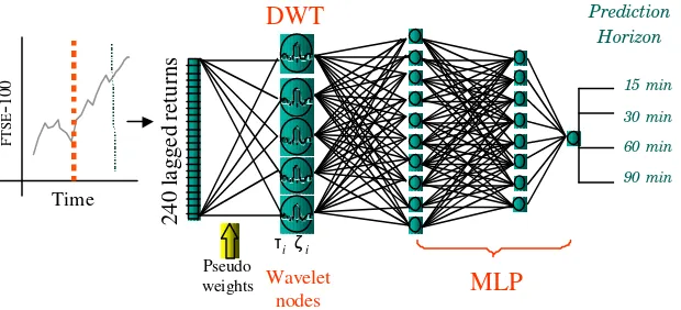
In this paper, we shall present a method of choosing a suitable set of child wavelets such that the transformation of the original data (the 240 lagged returns of the FTSE-100 Future) will enhance the non-linear separability of different classes of signal whilst significantly reducing the dimension of the data. We show how this may be achieved naturally by implementing the wavelet transform as a set of wavelet

neurons contained in the first layer of a multi-layer perceptron (Rummelhart et al [1986]) (henceforth R86). The shifts and dilations of the wavelet nodes are then found along with the other network parameters through the minimisation of a penalised least squares objective function.We then extend this concept to include automatic determination of a suitable number of wavelet nodes by applying Bayesian priors on the child wavelet parameters during training of the neural network and enforcing orthogonality between the wavelet nodes using soft constraints.

4

Wavelet Encoding A Priori Orthogonal Network

(WEAPON)

4.1 The Wavelet Neuron

The most common activation function used for neurons in the Multi-Layer Perceptron architecture is the sigmoidal activation function.

ϕ

( )

x

and the weighted connections between the neuron and the previous layer

ω

_{k i,} , i.e.

y

_i

x

Noting the similarity between Equations (6) and (4), we can implement the Discrete Wavelet Transform as the first layer of hidden nodes of a multi-layer perceptron (MLP). The weights connecting each wavelet node to the input layer

ω

_{j i,} must be constrained to be discrete samples of a particular wavelet child

φ

τ ζj j

i

,

( )

and the activation function of the wavelet nodes should be the identity transformation

ϕ

( )

x

=

x

. In fact, we may ignore the weights connecting the wavelet node to the previous layer and instead characterise the wavelet node purely in terms of values of translation and scale,

τ

and

ζ

. The WEAPON architecture is shown below in Figure 3.

We can note that, in effect, the WEAPON architecture is a standard four-layer MLP with a linear set of nodes in the first hidden layer and in which the weights connecting the input layer to the first hidden layer are constrained to be wavelets. This constraint on the first layer of weights acts to enforce our a

priori knowledge that the input components are not presented in an arbitrary fashion, but in fact have a defined temporal ordering.

4.2 Training the Wavelet Neurons

The MLP is usually trained using error backpropagation (backprop) [R86] on a set of training examples. The most commonly used error function is simply the sum of squared error over all training samples

E

D

Backprop requires the calculation of the partial derivatives of the data error

E

_D with respect to each of the free parameters of the network (usually the weights and biases of the neurons). For the case of the wavelet neurons suggested above, the weights between the wavelet neurons and the input pattern are not free but are constrained to assume discrete values of a part icular child wavelet.

The free parameters for the wavelet nodes are therefore not the weights, but the values of translation and dilation

τ

and

ζ

. To optimise these parameters during training, we must obtain expressions for the partial derivatives of the error function

E

_D with respect to these two wavelet parameters.

The usual form of the backprop algorithm is:

∂

y

, often referred to as

δ

j,is the standard backpropagation of error term, which may be

found in the usual way for the case of the wavelet nodes. The partial derivative

∂

∂ω

y

i j,

must be substituted with the partial derivatives of the node output y with respect to the wavelet parameters. For a given Mother wavelet

φ

(

x

)

, consider the output of the wavelet node, given in Equation (4). Taking partial derivatives with respect to the translation and dilation yields:

Using the above equations, it is possible to optimise the wavelet dilations and translations. For the case of the Mexican Hat wavelet we note that

φ

' ( )

t

π

t

(

t

)

e

Once we have derived suitable expressions for the above, the wavelet parameters may be optimised in conjunction with the other parameters of the neural network by training using any of the standard gradient based optimisation techniques.

4.3 Orthogonalisation of the Wave let Nodes

A potential problem that might arise during the optimisation of the parameters associated with the wavelet neurons is that of duplication in the parameters of some of the wavelet nodes. This will lead to redundant correlations in the outputs of the wavelet nodes and hence the production of an overly complex model.

One way of avoiding this type of duplication would be to apply a soft constraint of orthogonality on the wavelets of the hidden layer. This could be done through use of the addition of an additional error term in the standard data misfit function, i.e.

E

_W

where denotes the projection

f g

f i g i

In the previous section, backprop error gradients were derived in terms of the unregularised sum of squares data error term,

E

D. We now add in an additional term for the orthogonality constraint to yield

a combined error function M(W), given by

M W

(

)

=

α

E

D

+

γ

E

W

φ

(13)

Now, to implement this into the backprop training rule, we must derive the two partial derivatives of

E

W

φ

with respect to the dilation and translation wavelet parameters

ζ

_i and

τ

_i. Expressions for the partial derivatives above are obtained from (9) and are:

These terms may then be included within the standard backprop algorithm. The ratio

α

γ

determines the balance that will be made between obtaining optimal training data errors against the penalty incurred by having overlapping or non-orthogonal nodes. The ratio may either be either estimated or optimised using the method of cross validation.

The effect of the orthogonalisation terms during training will be to make the wavelet nodes compete

with each other to occupy the most relevant areas of the input space with respect to the mapping being performed by the network. In the case of having an excessive number of wavelet nodes in the hidden layer this generally leads to the marginalisation of a number of wavelet nodes. The marginalised nodes are driven to areas of the input space in which little useful information with respect to the discriminatory task performed by the network is present.

4.4 Weight and Node Elimination

The a priori orthogonal constraints introduced in the previous section help to prevent significant overlap in the wavelets by encouraging orthogonality. However, redundant wavelet neurons will still remain in the hidden layer though they will have been marginalised to irrelevant (in terms of discrimination) areas of the time/frequency space.

At best, these nodes will play no significant role in modelling the data. At worst, the nodes will be used to model noise in the output targets and will lead to poor generalisation performance. It would be preferable if these redundant nodes could be eliminated.

A number of techniques have been suggested in the literature for node and/or weight elimination in neural networks. We shall adopt the technique proposed by Williams (1993) and MacKay (1992a, 1992b) and use a Bayesian training technique, combined with a Laplacian prior on the network weights as a natural method of eliminating redundant nodes from the WEAPON architecture. The Laplacian Prior on the network weights implies an additional term in the previously defined error function (13), i.e.

W W

D

E

E

E

W

M

(

)

=

α

+

γ

φ

+

β

(15)

where

E

_W is defined as

∑

=

j i

j i W

E

,

,

ω

(16)

5

Predicting The FTSE-100 Future Using WEAPON

Networks

5.1 The Data

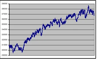
We shall apply the network architecture and training rules described in the previous section to the task of predicting future returns of the FTSE-100 index future quoted on LIFFE. The historical data used was tick-by-tick quotes of actual trades supplied by LIFFE (see Figure 4). The data was pre-processed to a 1-minutely format by taking the average volume adjusted traded price during each minute. Missing values were filled in by interpolation but were marked as un-tradable.

Minutely prices were obtained in this manner for 18 months, January 1995-June 1996, to yield approximately 200,000 distinct prices. The entire data set was then divided into three distinct subsets, training/validation, optimisation and test. We trained and validated the neural network models on the first six months of the 1995 data. The prediction performance results, quoted in this section, are the results of applying the neural networks to the second six mo nths of the 1995 data (optimisation set). We reserved the first 6 months of 1996 for out-of-sample trading performance test purposes.

2 9 0 0 0 3 0 0 0 0 3 1 0 0 0 3 2 0 0 0 3 3 0 0 0 3 4 0 0 0 3 5 0 0 0 3 6 0 0 0 3 7 0 0 0 3 8 0 0 0 3 9 0 0 0

Figure 4: FTSE -100 Future January 1995 to June 1996.

5.2 Individual Predictor Performances

Table 1 to Table 4 show the performances of four different neural network predictors for the four prediction horizons (15, 30, 60 and 90 minutes). The predictors used were

1. Simple early-stopping [Hecht-Nielsen[1989])] MLP trained using all 240 lagged return inputs with an optimised number of hidden nodes found by exhaustive search (2-32 nodes).

2. A standard weight decay MLP (Hinton [1987]) trained using all 240 lagged returns with the value of weight decay lambda optimised by cross validation.

3. An MLP trained with Laplacian weight decay and weight/node elimination (as in Williams [1993])

4. WEAPON architecture using wavelet nodes, soft orthogonalisation constraints and Laplacian weight decay for weight/node elimination.

The performances of the architectures are in terms of :

1. RMSE prediction error in terms of desired and actual network outputs.

3. Large turning point accuracy: This is the number of times that the network correctly predicts the sign of returns whose magnitude is greater than one standard deviation from zero (this measure is relevant in terms of expected trading system performance).

Prediction horizon % Accuracy Large % Accuracy RMSE

15 51.07% 54.77% 0.020231

30 52.04% 59.55% 0.039379

60 51.69% 54.61% 0.074023

90 51.12% 50.82% 0.085858

Table 1: Results for ML P using early stopping

Prediction horizon % Accuracy Large % Accuracy RMSE

15 50.75% 52.70% 0.022533

30 51.00% 56.08% 0.034591

60 53.35% 54.09% 0.060929

90 54.82% 57.24% 0.128560

Table 2: Results for weight decay ML P

Prediction horizon % Accuracy Large % Accuracy RMSE

15 51.25% 48.55% 0.020467

30 54.16% 54.34% 0.035261

60 46.14% 43.48% 0.064493

90 50.39% 50.82% 0.090002

Table 3: Results for L aplacian weight decay ML P

Prediction horizon % Accuracy Large % Accuracy RMSE

15 53.27% 57.43% 001879

30 52.79% 56.19% 0.03414

60 54.62% 57.94% 0.06044

90 55.11% 58.28% 0.08118

Table 4: Results for WE A PON

We conclude that the WEAPON architecture and the simple weight decay architecture appear significantly better than the other two techniques. The WEAPON architecture appears to be particularly good at predicting the sign of large market movements.

5.3 Use of Committees for Prediction

In the previous section, we presented prediction performance results using a single WEAPON architecture applied to the four required prediction horizons.

( )

( )

The weightings may either be simple averages (Basic Ensemble Method) or may be optimised using an OLS procedure (Generalised Ensemble Method). Specifically, the OLS weightings may be determined by

ρ

ρ

α =

_{Ξ Γ}

−1

(18)

where

Ξ

and

Γ

are defined in terms of the outputs of the individual trained networks and the training examples, i.e.

Below, we show the prediction performances of committees composed of five independently trained WEAPON MLPs, for each of the prediction horizons. We conclude that the performances (in terms of RMSE) are superior to those obtained using a single WEAPON architecture. Turning point detection accuracy, however, is broadly similar.

Prediction horizon % Accuracy Large % Accuracy RMSE

15 53.25% 57.27% 0.01734

30 53.14% 56.98% 0.03216

60 54.47% 57.71% 0.05592

90 55.19% 58.69% 0.08091

Table 5: Results for Committees of five independently trained WE A PON architectures.

6

The Signal Thresholded Trading System

6.1 Background

• What are the effective transaction costs that are incurred each time we execute a round-trip trade?

• Over what horizon are we making the predictions? If the horizon is particularly short term (i.e. 5-minute ahead predictions on intra-day futures markets) is it really possible to get in and out of the market quickly enough and more importantly to get the quoted prices? In terms of building profitable trading systems it may be more effective to have a lower accuracy but longer prediction horizons.

• What level of risk is being assumed by taking the indicated positions? We may, for instance, want to optimise not just pure profit but perhaps some risk-adjusted measure of performance such as Sharpe Ratio or Sterling Ratio.

An acceptable trading system has to take account of some or all of the above considerations.

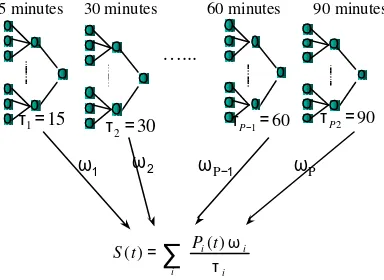
6.2 The Basic STTS Model

Assume we have P predictors making predictions about the expected FTSE-100 Futures returns. Each of the predictors makes predictions for

τ

_i time steps ahead. Let the prediction of the

i

th predictor at time t be denoted by

p t

i

( )

. We shall define the normalised trading signal

S t

( )

at time t to be:

S t

i

p t

i

i i

P

( )

=

( )

=

∑

ω

_τ

1

(20)

where

ω

_i is the weighting given to the

i

thpredictor. An illustration of this is given in Figure 5.

∑

=

i i

i i t

P t S

τ ω ) ( )

(

ω1 ωP−1 ωP

30 minutes 60 minutes 90 minutes

ω2

15 minutes

…...

15

1=

τ ₃₀

2=

τ τP−1=60 τP2=90

Figure 5: Weighted summation of predictions from four WE A PON committee predictors to give a single trading signal.

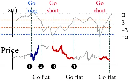
We shall base the trading strategy on the strength of the trading signal

S t

( )

at any given time t. At time t we compare the trading signal

S t

( )

with two thresholds, denoted by

α

and

β

. These two thresholds are used for the following decisions:

•

α

is the threshold that controls when to open a long or short trade.

At any given time t, the trading signal will be compared with the appropriate threshold using the current trading position. In particular, details of the actions defined for each trading position are found in Table 6:

Current position Test Action: Go... Flat if S(t) > α Long Flat if S(t) < -α Short Long if S(t) < -β Flat Short if S(t) > β Flat

Table 6: Using the trading thresholds to decide which action to tak e

Figure 6 demonstrates the concept of using the two thresholds for trading. The two graphs shown in Figure 6 are the trading signals

S t

( )

for each time t (top) and the associated prices

p t

i

( )

displayed in

the bottom graph. The price graph is coded for the different trading position that are recommended, thick blue and red lines for being in a long or short trading position, grey otherwise. At the beginning of trading we are in a flat position. We shall open a trade if the trading signal exceeds the absolute value of

α

. At the time marked _Πthis is the case since the trading signal is greater than

α

. We shall open a long trade. Unless the trading signal falls below -

β

, this long trade will stay open. This condition is fulfilled at the time marked _•, when we shall close out the long trade. We are now again in a flat position. At time _Ž the trading signal falls below -

α

, so we open a short trading position. This position is not closed out until the trading signal exceeds

β

, which occurs at time _• when the short trade is closed out.

s(t)

Price

α β

−α −β

Go long

Go short

Go short

Go flat Go flat Go flat

Œ • Ž

•

Figure 6: Trading signals and prices

7

Results

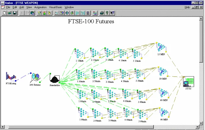
Figure 7: The Trading System for F TSE -100 futures. 240 lagged returns are extracted from the F TSE -100 future time series and after standardisation, input to the 20 WE A PON

predictors, arranged in four committes. E ach committee is responsible for a particular prediction horizon. The predictions are then combined for each committee and passed onto

the STTS trading module.

The optimal values for the STTS thresholds

α

and

β

and the four STTS predictor weightings

ω

_i to use were found by assessing the performance of the STTS model on the optimisation data (last 6 months of 1995) using particular values for the parameters. The parameters were optimised using simulated annealing (Kirkpatrick et al [1983]) with the objective function being the net trading performance (including transaction costs) on this period measured in terms of Sharpe ratio.

In terms of trading conditions, it was assumed that there would be a three minute delay in opening or closing any trade and that the combined bid -ask spread / transaction charge for each round trip trade would be 8 points. Both are considered conservative estimates. It was also assumed that contracts of the FTSE-100 future are rolled over on the delivery month, where basis adjustments are made and one extra trade is simulated.

After the optimal parameters for the STTS system were determined, the trading system was applied to the previously unseen data of the first six months of the 1996.

Table 7 summarises the trading performance over the six-month test period in terms of net over-all profitability, trading frequency and Sharpe Ratio.

Monthly net profitability in ticks ₅₃

Average monthly trading frequency (round-trip)

18

Sharpe ratio daily (monthly) _{0.136 (0.481)}

8

Conclusion

We have presented a complete trading model for adopting positions in the LIFFE FTSE-100 future. In particular, we have developed a system that avoids the three weaknesses that can be identified wit h many financial trading systems, namely

1. Data Pre-Processing – We have constrained the effective dimension of the 240 lagged returns by imposing a Discrete Wavelet Transform on the input data via the WEAPON neural network architecture. We have also, within the WEAPON architecture devised a method for automatically discovering the optimal number of wavelets to use in the transform and also which scales and dilations should be used.

2. Regularisation – We have applied Bayesian regularisation techniques to constrain the complexity of the neural network prediction models. We have demonstrated the requirement for this by comparing the prediction performances of regularised and unregularised (early-stopping) neural network models.

3. STTS Trading Model – The STTS model is designed to transform predictions into actual trading strategies. Its objective criterion is therefore not RMS prediction error but the risk adjusted net profit of the trading strategy.

The model has been shown to provide relatively consistent profits in simulated out-of-sample high frequency trading over a 6-month period.

9

Bibliography

[1] Buntine WL & Weigend AS (1991) Bayesian Back-Propagation,Complex Systems. 5, 603-643. [2] Casasent DP & Smokelin JS (1994) Neural Net Design of Macro Gabor Wavelet Filters for

Distortion-Invariant Object Detection In Clutter,Optical Engineering, Vol. 33, No.7, pp 2264-2270.

[3] Debauchies I (1988) Orthonormal Bases of Compactly Supported Wavelets, Communications in Pure and Applied Mathematics, Vol. 61, No. 7, pp 909-996.

[4] Fahlman SE (1988) Faster Learning Variations On Back-Propagation: An Empirical Study,

Proceedings Of The 1988 Connectionist Models Summer School, 38-51. Morgan Kaufmann. [5] Fukunaga K (1990), Statistical Pattern Recognition (2nd Edition) Academic Press.

[6] Hashem S & Schmeiser B (1993), Approximating a function and its derivatives using MSE-optimal linear combinations of trained feed-forward neural networks, Proc. world congress on Neural Networks, WCNN-93, I-617-620.

[7] Hecht-Nielsen R (1989), Neurocomputing, Addison-Wesley.

[8] Hinton, GE (1987), Learning translation invariant recognition in massively parallel networks. In JW de Bakker, AJ Nijman and PC Treleaven (Eds.), Proceedings PARLE Conference on Parallel Architectures and Languages Europe, 1-13, Springer-Verlag.

[9] Kirkpatrick S, Gelatt CD & Vecchi MP (1983) Optimization by simulated annealing. Science 220 (4598), 671-680.

[10]MacKay DJC (1992) Bayesian Interpolation. Neural Comput. 4(3), 415-447.

[11]MacKay DJC (1992) A Practical Bayesian Framework For Backprop Networks, Neural Comput. 4(3), 448-472.

[12]Meyer Y (1995) Wavelets and Operators, Cambridge University Press.

[14]Refenes AN, Azema-Barac M & Karoussos SA (1993), Currency Exchange Rate Prediction and Neural Network Design Strategies, Neural Computing and applications, 1 1 46-58.

[15]Rummelhart DE, Hinton GE & Williams RJ (1986) Learning Internal Representations By Error Propagation in Parallel Distributed Processing, Chapter 8. MIT Press.

[16]Shannon CE (1948), A mathematical theory of communication, the Bell System technical Journal, 27 (3), 379-423 and 623-656.

[17]Szu H & Telfer B (1992) Neural Network Adaptive Filters For Signal Representation, Optical Engineering 31, 1907-1916.

[18]Telfer BA, Szu H & Debeck GJ (1995) Time-Frequency, Multiple Aspect Acoustic Classification, World Congress on Neural Networks, Vol.2 pp II-134 – II-139.

[19]Toulson DL & Toulson SP (1996) Use Of Neural Network Ensembles for Portfolio Selection and Ris k Management, Proc Forecasting Financial Markets- Third International Conf, London.

[20]Toulson DL & Toulson SP (1996) Use of Neural Network Mixture Models for Forecasting and Application to Portfolio Management, Sixth Interntl Symposium on Forecasting, Istanbul.

[21]Weigend AS, Zimmermann H-G & Neuneier R (1996), Clearning. In Neural Networks in Financial Engineering, 511-522, World Scientific

[22]White H (1988), Economic Prediction Using Neural Networks: The Case of IBM daily Stock Returns, Proc. IEEE Int. conference on Neural Networks, San Diego, II-451-459.