Copyright @2018, Universitas Klabat Anggota CORIS, ISSN: 2541-2221/e-ISSN: 2477-8079
We have been always trying to predict the weather to minimize risk, produce strategy, and other decision making situation. To achieve this, monitoring method need to be used to gather data. Rainfall monitoring is one of the area that widely used and one of the mostly used method is satellite-based rainfall monitoring. However, there are limitation to apply to the Satellite Rainfall (SR) estimation specifically on its accuracy and lack of certainty. Thus, study that directed to measure the inaccuracies of SR measurements is needed by using data of distribution of Actual Rainfall (AR). The SR data is taken from the National Oceanic and Atmospheric Administration (NOAA)’s Hydro—Estimator while the AR data was from the National Institute of Water and Atmospheric Research (NIWA). Through the statistics and interpolation analysis using ArcGIS, the study shows a prominent result of SR estimation accuracy in the sample area and thus may opens up more similar implementation as well as stands as a good benchmark for future improvement of the method. This study also shows how interpolation method through a GIS software could provide a significant result on a geographical related studies.
Keywords : GIS, Geospatial Analysis, Interpolation Analysis, Arcgis
Abstract
Manusia terus mencoba untuk mengprediksi cuaca untuk mambantu dalam banyak hal seperti meminimalisir resiko, membuat strategi, dan keperluan pengambilan keputusan lainnya. Untuk mewujudkan ini sebuah metode pengawasan diperlukan untuk mengumpulkan data. Pengawasan hujan merupakan salah satunya dan metode berbasis satelit adalah salah satu yang paling banyak digunakan. Namun ada beberapa batasan yang di miliki sistem Satellite Rainfall (SR) dalam hal ketepatan dan kepastian. Maka dari itu, penelitian ini di arahkan untuk mengukur ketepatan dari SR dengan menganalisakan nya dengan data hujan sebenarnya atau Actual Rainfall (AR). Data SR di ambil dari badan National Oceanic and Atmospheric Administration (NOAA) sedangkan data AR diambil dari National Institute of Water and Atmospheric Research (NIWA). Melalui analisa statistik dan interpolasi menggunakan ArcGIS, studi ini menemukan signifikansi yang cukup baik dari ketepatan SR. Hal ini membuka jalan bagi implementasi yang serupa dan bisa menjadi standar benchmark yang baik untuk perbaikan di kemudian hari. Penelitian ini juga menunjukkan bagaimana metode interpolasi melalui software GIS bisa memberikan hasil yang baik untuk studi menyangkut geografis.
1. INTRODUCTION
Mankind have been trying to predict the weather for millennia. Since the nineteenth century the application of science and technology has been contributing to the advance of weather forecasting. In our daily live the information that gathered may be important in many fields such as transportation, agriculture and expedition. Mainly it may be used to minimize risk, produce strategy, and other decision making situation. To achieve this, monitoring method need to be used to gather data. Rainfall monitoring is one of the area that widely used and one of the mostly used method is satellite-based rainfall monitoring. The advantage of satellite-based monitoring is it can be used to observe both terrain and non-terrain area and able to cover the entire earth.
However, some limitation may apply to the Satellite Rainfall (SR) estimation specifically on its accuracy and lack of certainty. Thus, study that directed to measure the inaccuracies of SR measurements is needed. This begs the researcher a question: How accurate is satellite-based rainfall estimator?
A model that constructed to characterizes the distribution of Actual Rainfall (AR) from SR estimates may be one of the solution to the problem. This study will emulate the solution above to create a model and once a model has been formed, it will be evaluated and tested to generate rainfall measurement in non-observed area by using spatial interpolation method. ArcGIS will be used to process the calculation and interpolation part. First the more detailed research background and related literature will be discussed.
Rainfall data that gathered from two different sources. SR data were taken from the
National Oceanic and Atmospheric Administration (NOAA)’s Hydro-Estimator which is under the US Department of Commerce and AR data were acquired from National Institute of Water and Atmospheric Research (NIWA) database.
2. STATISTICAL ANALYSIS &INTERPOLATION
2.1 Statistical Analysis
To see how accurate or correlated SR to AR we need to measure their linear correlation.
To measure the linear correlation between AR and SR we may use the Pearson’s Correlation Coefficient or “r”. As depicted on Pearson’s Correlation Coefficient (1), this is the equation to find r, where X is SR as the predictor variable and Y is AR as the response variable.
𝑟 =
∑(𝑋𝑖−𝑋̅)(𝑌𝑖 −𝑌̅)[∑(𝑋𝑖−𝑋̅)2 ∑(𝑌𝑖 −𝑌̅)2]1/2 (1)
The value of r may have resulted between +1 and -1, where correlation on 1 is positive, -1 is negative, and 0 is none. Some samples of r values and on different scatter plots. [1]. Once we know how strong the relationship between the two variable, we may create regression model with error distribution that characterizes the conditional distribution of AR rate given SR estimates.
𝑎 =
(∑ 𝑦)(∑ 𝑥𝑛(∑ 𝑥22)− (∑ 𝑥)(∑ 𝑥𝑦))− (∑ 𝑦)2 (2)𝑏 = 𝑛(∑ 𝑥𝑦) − (∑ 𝑥) (∑ 𝑦)
Firstly, value of a and b are calculated with the equation (2), where N is the number of observations or instances, X is value of SR, and Y is value of AR. Then, the Regression equation would be formed as equation (3) below.
𝑦2= 𝑎 + 𝑏𝑥 + 𝑒 or 𝑌
𝑖 = 𝐵0+ 𝐵𝑖𝑋𝑖+ 𝑒𝑖 (3)
Where 𝐵𝑖𝑎𝑛𝑑 𝐵0 are the parameters (and 𝐵0is the yx-intercept), and i is the trial number
(1,…,n). [2 p. 23-26 ]. Once we have model we could determine how well the model fits the data by counting the R-squared (R2) value as shown on equation (4) where is the mean of the observed data and 𝑓𝑖 is the i-th function of i-th 𝑥𝑖. In this case the if the R value could get closer The purpose of interpolation on this case is to analyze the spatial distributions of both SR and AR and to evaluate the rainfall measurement in uncovered area then create a continuous dataset that could be portrayed over a map of the sampled area. There are three interpolation methods classification: local/global methods, deterministic/geostatistical methods, and exact/approximate methods.
According to Erdogan [4], deterministic/geostatistical are the most widely used ones
among the three classifications. Deterministic interpolation is constructed by the surrounding’s
degree of similarity such as in Inverse Distance Weighted (IDW) or degree of smoothing such as in Radial Basis Functions (RBF). On the other hand, geostatistical methods is based on statistical model that involve stastical relationship among the calculated points. Kriging is an example of geostatistical interpolation method.
As shown on figure 1, in the IDW method, each points may affect other unknown points and that influence fades with distance. Therefore, IDW assumes that area that are close to each other are similar and those that farther apart are more different. The IDW method should be applied where the points are dense enough around the area that going to be analyzed. The advantage of IDW, with enough dense positioned points, it can estimate values from flat area through extreme changes of terrains and cliffs area. However, IDW may not be accurate if the point value is beyond the maximum or minimum values. On the other side, RBF, another deterministic interpolation method, works quite similar with IDW but with a mathematical
function that create smooth the surface that passes through the points as illustrated on figure 2. It also can be observer that, unlike IDW, values below or above minimum or maximum can be identify. RBFs may be very useful and effective when producing surfaces such as elevation and not recommended when there are extreme differences between point (such as cliffs or fault lines) as the smoothing may not be effective.
Figure 2 “Smoothing” in RBF method [4]
2.3 Related studies
A similar study was conducted in China in 2002. Lin, MO, LI and LI [5] gathered 30 years of annual precipitation between 1961 and 1990. The data was gathered from 2114 stations and compared with its respective adjacent regions and analyzed using IDW method. The outcome was quite satisfying and accurate. A similar study was conducted by Mohamad Noor, Hussein Hassan and Yaseen Mustafa in 2014. Noori, Hassan and Mustafa [6] evaluates spatial estimation of rainfall distribution in Duhok Governorate, Iraq using GIS where the studies involve 25 stations and rainfall data that was gathered within 2000 and 2010. The studies used 25% of the total stations for cross-validation purpose and assume without data. The author concluded that the IDW method were able to predict the probable rainfall data for all the 25 rainfall stations. Nevertheless, the interpolation method may be used also on other case study such as estimating timberland productivity. Bridges [7], on his studies, were able to map spatially forest productivity in six productivity class by using ordinary kriging spatial interpolation method.
3. DATA COLLECTION
3.1 Actual Rain Data
NIWA’s Actual Rain data was gathered using a device called udometer or rain gauge.
The rain gauge measure amount of precipitation over a set period of time in millimeters (mm). There are several type of rain gauge, on NIWA The tipping bucket of rain gauge would activate a switch each time the water reach certain level. Each output represents 0.2mm of rainfall, thus accuracy level is within 2%, with intensity of rainfall at 100mm/hour. [8]
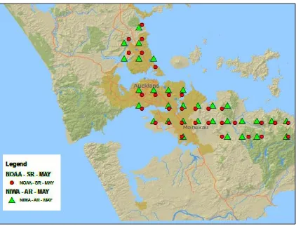
The rain gauge, along with other weather monitoring components, is installed on the NIWA climate stations that spread across New Zealand. The station is manufactured, installed and maintained to World Meteorological Organization (WMO) standards. The data is gathered from 31 points in Auckland Central, North Shore, and Manukau.
The actual rain data was obtained from NIWA’s Climate database
The data consist of several grids/columns, but the ones that are used are
“Station”, which is the ID of the station,
“Rain (mm)”, which shows the total (not average) of rain per day (24-hours) in millimeter in the rain gauge. The collection starts from 9am through 9am the next day local times.
“Date” indicates when the data is gathered in local times (UTC+12).
In the form of excel files, the gathered data was from 2 selected months. 1 February 2013 through 28 February 2013 and 1 May 2013 through 31 May 2013, giving total of 868 lines for February (28 days x 31 stations) and 961 lines for May (31 days x 31 stations).
3.2 Satellite Data
The satellite-based rainfall estimator system is based on hydro-estimator (H-E) which
uses infrared (IR) data from the NOAA’s Geostationary Operational Environmental Satellites
(GOES). It was intended to provide critical rainfall data over oceans and sparsely populated regions where data gauges or radar-based information are not available or reliable [9] . At NOAA, the H-E estimates have been used since the late 1970’s. At first it was used for the Interactive Flash Flood Analyzer [10], before it was used as fully automated Auto-Estimator Vicente, Scofield and Menzel [11]. The current-generation operational algorithm at NESDIS is the Hydro-Estimator (H-E) which has been used since 2002 [12].
The hydro estimation works by IR data’s pixel, or T, as input which is processed in a special
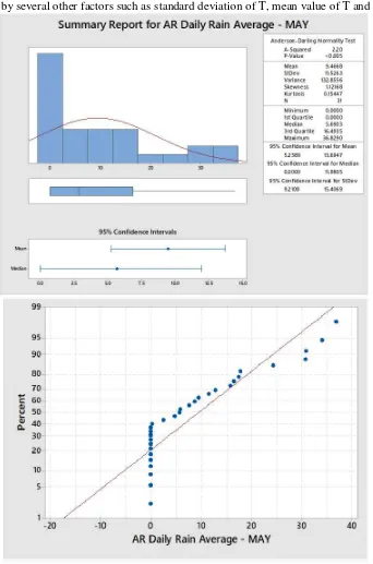
by several other factors such as standard deviation of T, mean value of T and
Figure 4 Summary Report of AR
Numerical Weather Prediction (NWP) rate. The data is gathered from chosen 31 points
to the nearest to NIWA’s points across Auckland City, North Shore, and Manukau.
The satellite rain data was acquired from the NOAA (STAR) – Hydro-estimator website (https://www.star.nesdis.noaa.gov/smcd/emb/ff/digGlobalData.php).
Total of 31 points are selected corresponding to the nearest NIWA’s AR station location as
Figure 5 Summary Report of SR
The data comes in the form of text file with only one column. One file contains one hour of rain data in mm of 24,891,111 (8001 x 3111 latitude/longitude grid) points of the entire earth. One value for each line and all in one single column. A total of 744 (24 hours x 31 days)
files for May 2013 and 672 (24 hours x 28 days) files for February 2013. There’s also a
metadata that specify the latitude/longitude coordinate for each lines of the data file. However, there are several missing files/hours (not available to be downloaded) thus the total number files is not exact.
KB, therefore a total of around 126 GB, for May, and 114 GB, for February, of data is being processed. Each value need to be applied with the formula R = (value-2) * 0.30, where value is the raw value of data and R is the measured rain in mm. The rain data is summed up for each
day so it would have the same structure as the AR data. The SR data columns are: “Nearest Station”, “Rain (mm)”, and “Date”.
4. RESULT &DISCUSSION
4.1 Statistical & Graphical Result
The statistical result of the studies including individual report, regression analysis and Pearson Coefficient are discussed on this section. Figure 4 and 5 shown the summary graphical
and statistic data AR and SR’s daily rain average. There’s no SR data on February 2013 as the gathered value all are resulted in 0 mm and no values. From this point forward February data would not be analyzed.
Next are the comparison graphs where SR as the predictor (x) and AR as the response (y). Figure 6 shows the regression lines, confidence interval, prediction interval, and the
regression equation. Figure 7, in the other hand, shows the residuals’ histogram and normality
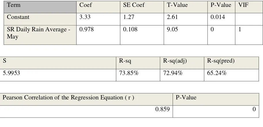
plot. Meanwhile, table 1 shows the regression coefficient values and the Pearson Correlation (r) value and table 2 shows unusual observations.
Table 1 Regression Coefficient and Pearson Correlation Value
Term Coef SE Coef T-Value P-Value VIF
Pearson Correlation of the Regression Equation ( r ) P-Value
0.859 0
Table 2 Fits and Diagnostics for Unsual Observations
Figure 6 Regression Line with CI & PI
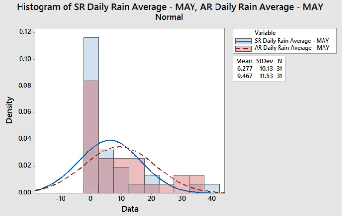
Figure 8 shows the density of both data, while figure 9 shows the scatter plot of both data on the Y-axis against date on the X-axis with regression lines.
4.2 Statistical & Graphical Analysis
Individual summary report of AR & SR, on figure 4 & 5, shown P-value less then < 0.005 this was caused by there are so many days are without rain (0 values), thus normal curve
distribution isn’t achieved. However, there can be seen that both data have somewhat follow
similar pattern.
Figure 8 Desnsity SR & AR
These similar patterns can be seen more visibly on figure 8. Though doesn’t have quite normal Gaussian distribution, yet the density histogram shows corresponding pattern which also supported by the close mean and standard deviation. On the other hand, on figure 9, scatterplot with regression lines of both data (Y-axis) against date (x-axis) shows quite related line. However, when analyzed together on the regression graph as depicted on figure 6, we could see how the regression line fit quite well, this also indicated with R2 value of 73.8%, a fairly high result. Moreover, with p-value of 0, that means the predictor (SR) is significant. This also
supported by the Pearson Correlation Coefficient or “r” value of 0.812 with the p-value of 0 as presented on table 1.
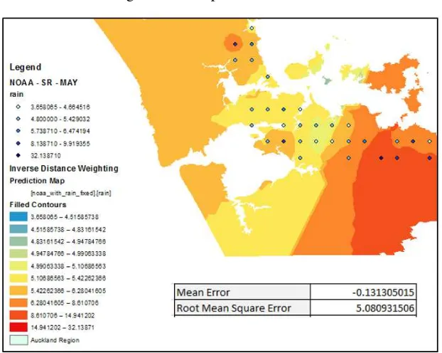
4.3 Interpolation Result and Analysis
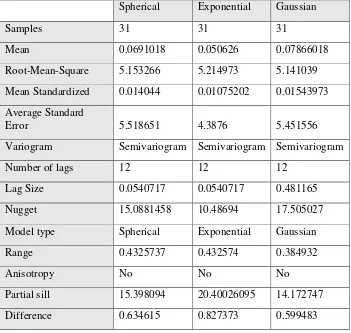
Total of two interpolation methods are applied using the ArcMap Software: Radial Basis Functions (RBF) and Inverse Distance Weighing (IDW). To identify the possible spatial structure of the total rain, we proceed with cross validation calculation. The best model was selected based on four indicators: 1. the Standardized Mean has to be near 0, 2. Smallest RMSE, 3. The average standard error mean closest to RMSE, 4. The Standardized Root-Mean-Squared nearest to one. Both interpolation shows great result with mean error very close to 0 with Gaussian model slightly top the other two model. These can be observed on Table 3 and maps on figures 10 and 11.
Tabel 3 Cross Validation
Spherical Exponential Gaussian
Samples 31 31 31
Mean 0.0691018 0.050626 0.07866018
Root-Mean-Square 5.153266 5.214973 5.141039
Mean Standardized 0.014044 0.01075202 0.01543973
Average Standard
Error 5.518651 4.3876 5.451556
Variogram Semivariogram Semivariogram Semivariogram
Number of lags 12 12 12
Lag Size 0.0540717 0.0540717 0.481165
Nugget 15.0881458 10.48694 17.505027
Model type Spherical Exponential Gaussian
Range 0.4325737 0.432574 0.384932
Anisotropy No No No
Partial sill 15.398094 20.40026095 14.172747
Figure 10 Interpolation with RBF
Figure 11 Interpolation with IDW
5. CONCLUSION
There are several limitations that need to be addressed regarding data gathering and accuracy. There are several hourly data from NOAA websites that cannot be included within the
analysis. This was caused either of “no-data” which is 0 value (2 means no rain) or “missing
data” where the file is not available. Though the corresponding data on NIWA has been
adjusted, however this may contribute to some slight shift of result.The location of the NOAA point is selected to the nearest NIWA station, yet they may not exactly on the same place, especially if it involves elevation, hence it may contribute to some loss of precision
well as stands as a good benchmark for future improvement of the method. This study also shows how interpolation method through a GIS software could provide a significant result on a geographical related studies.
There are plenty of room for future studies. By using the same method we could utilize other institutions data such as from Australia’s Bureau of Meteorology or United Kingdom’s Center of Ecology and Hydrology and compare their accuracies. From that we would have known which institutions would have better method for gathering actual rainfall data. Another possible follow through would be analyse and improve the result with methods interpolation method such as kriging and spline.
REFERENCES
[1] J. Lee Rodgers, and W. A. Nicewander, “Thirteen ways to look at the correlation
coefficient,” The American Statistician, vol. 42, no. 1, pp. 59-66, 1988.
[2] J. Neter, M. H. Kutner, and W. Wasserman, Applied linear statistical models: Richard D. Irwin, Inc., 1983.
[3] D. Algarni, and I. Hassan, “Comparison of thin plate spline, polynomial C-Function and Shepard's interpolation techniques with GPS derived DEM.,” Internation Journal of Applied Earth Observation and Geoinformation, vol. 3, no. 2, 2001.
[4] S. Erdogan, “A comparision of interpolation methods for producing digital elevation
models at the field scale,” Earth surface processes and landforms, vol. 34, no. 3, pp. 366-376, 2009.
[5] Z.-h. Lin, X.-g. MO, H.-x. LI, and H.-b. LI, “Comparison of Three Spatial Interpolation
Methods for Climate Variables in China [J],” Acta Geographica Sinica, vol. 1, pp. 005, 2002.
[6] M. J. Noori, H. H. Hassan, and Y. T. Mustafa, “Spatial Estimation of Rainfall
Distribution and Its Classification in Duhok Governorate Using GIS,” Journal of Water Resource & Protection, vol. 6, no. 2, 2014.
[7] C. A. Bridges, “Technical Note: Estimating Forest Site Productivity Using Spatial
Interpolation,” Southern journal of applied forestry, vol. 32, no. 4, pp. 187-189, 2008. [8] NIWA. "Climate stations and instruments," 26 May, 2018;
https://www.niwa.co.nz/our-services/instruments/instrumentsystems/products/climate-stations.
[9] NOAA. "STAR Satellite Rainfall Estimates - Hydro-Estimator," 25 May, 2018; https://www.star.nesdis.noaa.gov/smcd/emb/ff/HydroEst.php.
[10] R. A. Scofield, “The NESDIS operational convective precipitation-estimation
technique,” Monthly Weather Review, vol. 115, no. 8, pp. 1773-1793, 1987.
[11] G. A. Vicente, R. A. Scofield, and W. P. Menzel, “The operational GOES infrared
rainfall estimation technique,” Bulletin of the American Meteorological Society, vol. 79, no. 9, pp. 1883-1898, 1998.
![Figure 1 How IDW interpolation works [4]](https://thumb-ap.123doks.com/thumbv2/123dok/1943523.1591555/3.595.99.518.474.617/figure-how-idw-interpolation-works.webp)
![Figure 2 “Smoothing” in RBF method [4]](https://thumb-ap.123doks.com/thumbv2/123dok/1943523.1591555/4.595.194.401.175.284/figure-smoothing-rbf-method.webp)