Chp04 – Further Topics on Random Variables

Introduction to Probability

SECOND EDITION

Dimitri

P.

Bertsekas and John N. Tsitsiklis

Massachusetts Institute of Technology

WWW site for book information and orders http://www.athenasc.com

4

Further Topics

on Random Variables

Contents

4 . 1 . Derived Distributions . . . .

. p. 202

4.2. Covariance and Correlation . . .

. p. 217

4.3. Conditional Expectation and Variance Revisited

. p. 222

4.4. Transforms . . .

. p. 229

4.5. Sum of a Random Number of Independent Random Variables p. 240

4.6. Summary and Discussion

. p. 244

Problems . . . p. 246

202 Further Topics on Random Variables Chap. 4

In this chapter. we develop a number of more advanced topics. We introduce

methods that are useful in:

(

a

)

deriving the distribution of

a

function of one or multiple random variables;

(

b

)

dealing with the sum of independent random variables. including the case

where the number of random variables is itself random;

(

c

)

quantifying the degree of dependence between two random variables.

With these goals in mind. we introduce a number of tools. including transforms

and convolutions. and we refine our understanding of the concept of conditional

expectation.

The material in this chapter is not needed for Chapters

5-7.

with the ex­

ception of the solutions of a few problems. and may be viewed as optional in

a

first reading of the book. On the other hand, the concepts and methods dis­

cussed here constitute essential background for a more advanced treatment of

probability and stochastic processes. and provide powerful tools in several disci­

plines that rely on probabilistic models. Furthermore, the concepts introduced

in Sections

4.2 and 4.3

will be required in our study of inference and statistics,

in Chapters

8

and

9.

4.1 DERIVED DISTRIBUTIONS

In this section, we consider functions

Y

=

g(X)

of a continuous random variable

X.

We discuss techniques whereby, given the PDF of

X,

we calculate the PDF

of

Y

(

also called a

derived distribution).

The principal method for doing so is

the following two-step approach.

Calculation of the PDF of a Function Y

=

g(X) of a Continuous

Random Variable X

1 . Calculate the CDF

Fy

of

Y

using the formula

Fy(y)

=

P (g(X)

<

y)

=

fx(x) dx.

I g(x)Sy}

2.

Differentiate to obtain the PDF of

Y:

dFy

fy(y)

=

_{dy (y).}

Example

4.1. Let

X

be uniform on

[0. 11.

and let

Y

=

v'X.

We note that for every

_y

E

[0, 11.

we have

Sec. 4. 1 Derived Distributions

Example

4.2. John Slow is driving from Boston to the New York area, a distance of 1 80 miles at a constant speed, whose value is uniformly distributed between 30 and 60 miles per hour. What is the PDF of the duration of the trip?

on

4 . we

{

O. if y <

if 3 < y < O. if 6 <

1

x

. . . .

3 6 _y

4 . 1 : _{The calculation of t h e} P D F _{of Y ::::::} arrows i nd icate t he Row of the calculation .

3 6

y

4. 1

now

see Fig.

- 2

on

for

a

Y is

a linear function

9

4.2: The P D F _of aX _{+ b in terms of t he} PDF X . _{I n this figure}, a _{= 2} we obtain the PDF of aX . The range of Y is wider tha.n

a factor of a . t h e P D F must

this factor. But in order to the total area under the P DF to 1 , we need to scale dow n the P D F _{by the same factor a . The}

random variable aX + b is the same as aX except t hat its val ues are sh i fted by

b. Accordingly, we take t he P D F _{of aX and shift it ( horizontally) by b. The e nd}

result of these operations is the P D F _{of Y = aX + b an}d is given mat hemat ical ly

b) .

I f a were would be the same

of X would first need to be reflected around the vert ical axis ( ) yield ing

a horizontal and vertical ( by a factor of l a l l / i a l .

respec-the P DF _{of - l a l X} = aX . a horizontal sh ift of b would

the P_DF _{of + b.}

a a

be

a

with

y =

b,

a b are a O . Then,

206 Further Topics on Random Variables Chap. 4

To verify this formula, we first calculate the CDF of

Y

and then differenti­

ate. We only show the steps for the case where

a

>

_{OJ the case}

a

<

_{0 is similar.}

We now differentiate this equality and use the chain rule, to obtain

dFy

1

(

y

_-

b)

fy(y)

=

dy (y)

=

_�fx

_.

Example

4.4. A

Linear Function of an Exponential Random Variable.

Suppose that

X

is an exponential random variable with PDF

fx (x)

=

{

>'e-AX ,

if

x

�

�,

parameter >.

_/a

. In general, however,

Y

need not be exponential. For example, if

a

<

°

and

b

=

0, then the range of

Y

is the negative real axis.

Example

4.5. A

Linear Function of a Normal Random Variable is Nor­

mal.

Suppose that

X

is a normal random variable with mean

J-L

and variance

a2,

Sec. 4. 1 Derived Distributions 207

The Monotonic Case

The calculation and the formula for the linear case can be generalized to the

case where 9

is a monotonic function. Let

X

be a continuous random variable

and suppose that its range is contained in a certain interval I, in the sense that

fx (x) = 0

for

x

�

I. We consider the random variable Y

=

g(X),

and assume

that

9

is

strictly monotonic

over the interval I. so that either

(

a

)

g(x)

<

g(x')

for all

x. x'

E

I satisfying

x

< x' (

monotonically increasing

An important fact is that a strictly monotonic function can be "inverted"

in the sense that there is some function h, called the inverse of

g.

such that for

all

x

E

I, we have

y = g(x)

if and only if

x = h(y) .

For example, the inverse of the function

g(x) = 180/x

considered in Example 4.2

is

h(y) = 180/y,

because we have

y = 180/x

if and only if

x

=

180/y.

Other

such examples of pairs of inverse functions include

g(x) = ax + b.

For strictly monotonic functions

g,

the following is a convenient analytical

formula for the PDF of the function Y

= g(X).

PDF Formula for a Strictly Monotonic Function of a Continuous

Random Variable

Suppose that 9

is strictly monotonic and that for some function h and all

x

in the range of

X

we have

Further _on 4

that

h

is the in the region where

fy(y)

> 0 is given by

(y)

=

(h(y)) -(y) .

a verification of the above formula, assume first that 9 monotonical1y Then. we have

Fy(y)

=

P (g(X) �

y)

=

P (X

�

h(y))

=

Fx(h(y))�

where t he second equality can be justified the monotonically increasing property of 9 (see Fig. 4 .3) . By differentiating this relation , using also the chain

rule, we obtain

(y)

=

- (y)

=

(h(y)) - (y) .

dh

Because 9 is monotonically increasing.

h

is monotonically i ncreasing: so

Idh

dy

(y)

=

dy (y)

for a monotonically function

case

instead the relation

Fy(y)

=

(g(X)

$

y)

=

p(X

�

h(y))

= 1

-use the chain rule.

9 =

IS

(h(y)) .

4 . 3 : _{Calculating the probability}

p(g(X)

� _y

)

_{. Whe}

n

_{9 is}

(left . the event

{g(X)

� y } is the s

a

me as the event

{X

� h(y)}.

When 9 is (right the event � _y} is the

same as the event

{X

� h(y)}.

Sec. 4 . 1 Derived Distributions 209

variable on the interval

(0, 1].

Within this interval,

9

is strictly monotonic, and its

inverse is

h(y)

=

..;Y.

Thus, for any

y

E

(0. 1],

we have

We finally note that if we interpret PDFs in terms of probabilities of small

intervals, the content of our formulas becomes pretty intuitive; see

Fig. 4.4. Functions

of Two Random Variables

The two-step procedure that first calculates the CDF and then differentiates to

obtain the PDF also applies to functions of more than one random variable.

Example

4.7.

Two archers shoot at a target. The distance of each shot from the

center of the target is uniformly distributed from

0

to

1,

independent of the other

shot. What is the

PDF

of the distance of the losing shot from the center?

Let X and

Y

be the distances from the center of the first and second shots.

respectively. Let also

Z

be the distance of the losing shot:

Z

=

max

{

X,

Y}.

We know that X and Y are uniformly distributed over

[0. 1],

so that for all

z

E

[0. 1].

we have

on

.Ii

4.4: I llustration of the PDF _{a func­}

g. Consider an interval w here is a small number.

9. the of t his i nterval is another i nterval y +

is the of g� we have

or i n terms of the i nverse

We now note that t he event

y + _{} .}

dh - � - (y) ,

� X � x + } is the same as the event

� ::; V ::; y +

= � X ::; x +

We move to obtain

to the left- h and side and use our earlier formul a t h e ratio

=

i f we move side and use we obtain

x we _{z E}

= =

= < <

U nder Since

4. 1

4 . 5 : The calculation of the CDF of Z = Y / X i n 4 . 8 . The value P ( Y / X � is to shaded subarea of unit square. The figure on left deals with the case where 0 ::; z ::; 1 and t he on the refers to the case w here z > 1 .

Differentiating, we obtain

fz

=

{ 2Z'

_0, if O ::; z � l !

Y/X?

2 1 1

We wi l l find t he PDF of Z by first finding its CDF and then d ifferentiating.

cases 0 � z � 1 z > 1 . in we

= _{( X ::;; z)} =

{

1 - 1 / (22) I if z > I ,

2/2,

if 0

� 2 �

1 ,

0, otherwise.

By differentiating, we obtain

if O � z ::; l ,

if z > 1 ,

y

o

Further Topics on Variables

- y ... z

2: x x

4.6: The calculation of the of Z = X -

Y

in To obtain the value

- Y

> z ) we must integrate the joint P D F y

over the shaded area in t he above figures, which correspond to z � 0

side) and z < 0 (right side) .

z � O� we (see

(4) = -

Y

::; z

)

= 1

-

P (X

-

Y

>

=

1

-1""

dy

=

1 - e-'"

1x

1 1

-AZ

=

-

2"e .

For the case z < O, we can use a calculation , but we can also

4

symmetry. Indeed , the sym metry of the situation implies that the random

= - Y = same

(z)

= P ( Z _::;:

z

₎

=

P ( - Z �

-z)

= P ( Z � - z

)

= 1

-z < 0, we - z > °

Fz (z)

=

1 -

(-z)

₌

1 - (1 - �e-A(-Z))

₌

�eAZ.

Combining the two cases z � ° and z < 0, we obtain

( z ) =

{I

-

�e-AZ.

if z ;::: 0 ,

1

AZ

_f

2"e ,

i z < 0,

Sec. 4.1

Sums of Independent Random Variables - Convolution

We now consider an important example of a function

Z

of two random variables,

namely, the case where

Z

=

X

+ Y. for independent

X

and Y. For some initial

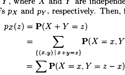
Suppose now that

X

and Y are independent continuous random variables

with PDFs

fx

and

fy,

respectively. We wish to find the PDF of

Z

=

X

+

Y.

where the third equality follows from the independence of

X

and Y. By differ­

entiating both sides with respect to

z,

we see that

fZlx(z

I

x)

=

fy(z -x).

Using

the multiplication rule, we have

Further Topics on Randonl Variables Chap. 4

(0,3)

. (1

• ( 2. 1 )

(:3.0)

,1'

4.7: The p z (3) that X + Y = 3 is the sum of the

of all such that x + y = 3, which are the in the figure.

The probability of a generic such point is of the form {x, 3 - = px { x )py ( 3

-we finally obtain

(z)

=

1:

(x, z)

(x)fy (z - x)

is entirely analogous to the one for the

by an the _PrvIFs are

except that by _PDFs.

and Y are independent and uniformly Z == + Y is

( z)

=

1:

o S z -

x

S 1 . two

max {O, Z -

I }

::; x :s; min { l ,

z}.

Thus,

(z) =

{

0,

1 , z} - z - l } , O ::; z ::;

::; x ::; 1 and

IS nonzero

which has the triangular shape shown in Fig. 4 . 9 .

4. 1

+ y

4.8: Illustrat ion of the convolution formul a for the case of cont i nuous

random with For smal l 6 , the of the

is

� x + y z +

= dx

� dx.

Thus.

The desired formula follows t. from bot h _{sides .}

1

o

random

1 2 z

z

ex p

{

- exp

{

can

answer turns out to

+

4. 1

ra_ndom

4 . 8 : _{I llustration of the convolution formula for the case of continuous}

with For small 6� the of the

indicated in the is :S X + Y :S .z + � ( Z )d .

z +

(y) dy dx

dx.

The desi red formula fol lows 6 from both sides.

1

o

4 . 9 : _{The PDF of the surn}

of two uniform

1 2 z

z + Y .

exp

{

_

(x

-

J.lx)2

exp

{

ax

2a;

can

answer turns out to

exp

{

2 1 5

216 Further Topics on Random Variables Chap. 4

which we recognize as a normal

PDF

with mean

/-Lx + _/-Ly

and variance

a; + a�.

We therefore reach the conclusion that the sum of two independent normal random

variables is normal. Given that scalar multiples of normal random variables are

also normal

(

cf. Example 4.5

)

, it follows that

aX +

bY is also normal, for any

nonzero

a

and b. An alternative derivation of this important fact will be provided

in Section 4.4, using transforms.

Example

4. 1 2.

The Difference of Two Independent Random Variables.

The convolution formula can also be used to find the

PDF

of

X

-

Y, when

X

and

Y are independent, by viewing

X

-

Y as the sum of

X

and -Y. We observe that

the

PDF

of -Y is given by f-Y (Y)

=

fy (-y),

and obtain

fx -y {z)

=

I:

fx {x)f-y{z - x) dx

=

I:

fx {x)fy {x - z) dx.

As an illustration, consider the case where

X

and Y are independent expo­

nential random variables with parameter

A,

as in Example 4.9. Fix some

z

�

0

and

in agreement with the result obtained in Example 4.9. The answer for the case

z

<

0

is obtained with a similar calculation or, alternatively. by noting that

fx -y {z)

=

fy-x {z)

=

f-(x-y) {z)

=

fx - y {-z),

where the first equality holds by symmetry, since

X

and Y are identically dis­

tributed.

When applying the convolution formula, often the most delicate step was

to determine the correct limits for the integration. This is often tedious and

error prone, but can be bypassed using a graphical method described next.

Graphical Calculation of Convolutions

We use a dummy variable

t

as the argument of the different functions involved

in this discussion; see also Fig. 4. 10. Consider two PDFs

fx(t)

and

fy(t).

For

a fixed value of

z,

the graphical evaluation of the convolution

(h)

(c)

2 1 7

(

z

)

amount z we are we any z .

b t c d t

-d - c

t

o _b

2 1 8 on

of two random

is defined by

Y) = [ (X - E[X]) (Y - )] .

When cov(X. Y) == O. \ve

i ng. a or

- E[Y

]

obtained in a

single

experiment -'tend" to

1 1).

Thus the

an of relationship

y y

negatively correlated

Here. X _{and Y are over the shown in the}

case ( a) t he covariance cov (X. Y ) is positive , while in case (b) it is

An f

o

r

m

ul

a

the

is

cov(X, Y) = E[X Y

J

- E [X] E [YL

as can be verified by a simple calculation. We a few

ances that are derived the definition: for any

and Z, and scalars a

b,

we have

cov(X. ) ==

cov( +

b)

== a .

cov(X.

)

.

V) :

cov(X. Z) .

4

Y) .

provides

and are independent , we E[X Y] = E [X] E [Y], which

following example.

Y) = O. Thus, if Y are independent ,

the converse is not true, as the

Example 4. The pair of random variables (X. Y) takes the values ( 1 , 0) , (0, 1 ) .

4 . 2 Correlation

Y are 0, =

E[Y]

= O.

for all pairs (x, y) ! either x or y is equal to 0, which implies that

XY

== 0 and

E[XY]

== O. Therefore,

Y) ==

Y are are not

example, a nonzero value of

X

fixes the value of

Y

to zero.

This example can generalized . assume and satisfy

E[X

I Y ==

yj

==

E[XJ ,

for all

y.

Then, assuming X and Y are discrete, t he total expectation theorem implies t hat

so

E[XY] ==

YPy

(y)E[X I Y ==

y]

== E[X]

ypy(y)

= E [X] E[YL

y

Y are uncorrelated , The argument for continuous case is similar.

The

x

4. 1 2 : Joint _PMF of X and Y

for Example 4 . 13. Each o f t h e four Here

p(X, Y)

of two random

as

cov(X,

Y )

version of

Y

i n

problems) .

- 1 to 1 (see

to

p

the > 0 same (or opposite, (or

p

< O) � of

X - E[X]

The size of

_Ipi

measure of extent to this is true. In a

that

if and Y

have

positive it

can be

shown that p = 1 (or

_p

= - 1 )

only if there exists _a positive (or c such

220 Further Topics on Random Variables Chap. 4

(see the end-of-chapter problems) . The following example illustrates in part this

property.

Example 4. 14.

Consider

n

independent tosses of a coin with probability of a head

equal to

p.

Let X and Y be the numbers of heads and of tails, respectively, and let

us look at the correlation coefficient of X and Y. Here, we have X

+

Y

=

n,

and

also E[X]

+

E[Y] =

n.

Thus,

X - E[X]

=

- (Y - E[Y]).

We will calculate the correlation coefficient of X and Y, and verify that it is indeed

equal to

-1.

We have

cov(X, Y) = E

[

(X E[X]) (Y

E

[Y])

]

=

-E

[

(X - E[X])

2]

= -var(X).

Hence, the correlation coefficient is

p(X, Y) = cov(X, Y)

_

Variance of the Sum of Random Variables

-1.

The covariance can be used to obtain a formula for the variance of the sum

of several (not necessarily independent) random variables. In particular, if

Xl , X2, . . . , Xn are random variables with finite variance, we have

and, more generally,

n

=

I:

var(Xi ) +

I:

COV(Xi, Xj ) .

i=l

{ (i,j) I

_{i,cj }}

Sec. 4.2 _{Covariance and Correlation}

n n

=

L L E[XiXj]

i=l j=l

n

=

L E [X/]

+

L E[XiXj]

i=l

_{(i,j)

I

i;ej}

n

=

L

v

ar

(

X

d

+

L

COV(Xi, Xj).

i=l

_{(i,j)

I

i;ej}

The following example illustrates the use of this formula.

221

Example

4.15.

Consider the hat problem discussed in Section 2.5, where

n

people

throw their hats in a box and then pick a hat at random. Let us find the variance

of X, the number of people who pick their own hat. We have

X

=

Xl

+ . . . +

X

_n

,

where Xt is the random variable that takes the value

₁

if the ith person selects

his/her own hat, and takes the value

0

otherwise. Noting that Xi is Bernoulli with

parameter

p

=

P(Xi

=

1)

=

l

/

n

, we obtain

For

i

=/:. j, we have

Therefore,

E[XiJ = �,

var(Xd

_{= � (1 - �) .}

1 1

=

P(Xi

_{= 1}

and Xj

= 1)

-

.

-n -n

1

=

P(Xi

=

I)P(Xj

_{= 1 1}

Xi

_{= 1) -}

-

_n2

1 1

1

n

=

L

var(Xt)

+

L

cov(Xi, Xj)

i=l

_{(i,j)

I

ii=j}

= n .

�

(1

- �)

+ n

(

n

-

1) . 1

n n n2

(

n

- 1)

222 Further Topics on Random Variables Chap. 4

Covariance and Correlation

•

The

covariance

of X and Y is given by

cov(X, Y)

= E

[

₍

_{X -}

E

[X

]

) (

Y -

E

_l

Y

]

₎

_]

=

E[XY] -

E

[X

]

E

[Y

]

. •

If cov(X, Y)

= 0,

we say that X and Y are

uncorrelated.

•

If X and Y are independent, they are uncorrelated. The converse is

not always true.

•

We have

var{X

+

Y)

=

var{X)

+

var{Y)

+

2cov{X, Y).

•

The

correlation coefficient

p{X, Y) of two random variables X and

Y with positive variances is defined by

and satisfies

p(X, Y)

=

cov(X, Y)

_{. ,}

-1 � p( X, Y) � 1.

4.3

CONDITIONAL EXPECTATION AND VARIANCE REVISITED

In this section, we revisit the conditional expectation of a random variable X

given another random variable Y, and view it

as

a random variable determined

by Y. We derive a reformulation of the total expectation theorem. called the

law of iterated expectations.

\Ve also obtain a new formula, the

law of total variance,

that relates conditional and unconditional variances.

We introduce a random variable, denoted by E[X I YJ, that takes the value

E[X I Y

=

y]

when Y takes the value

y.

Since E[X I Y

=

y]

is a function of

y,

E[X I Y] is a function of Y. and its distribution is determined by the distribution

of Y. The properties of E[X I Y] will be important in this section but also later,

particularly in the context of estimation

and

statistical inference, in Chapters 8

and

9.

Sec. 4.3 _{Conditional Expectation and Variance Revisited 223}

Since

E[X I

Yl

is a random variable, it has an expectation

E [E[X I

YJ]

of

its own, which can be calculated using the expected value rule:

L E[X

I Y

=

_{Ylpy (y) ,}

Y discrete,

E [E[X I

YlJ

y

I:

E[X

I Y

=

_{ylJy (y) dy,}

Y continuous.

Both expressions in the right-hand side are familiar from Chapters

2

and 3, re­

spectively. By the corresponding versions of the total expectation theorem. they

are equal to

E[Xl.

This brings us to the following conclusion. which is actually

valid for every type of random variable

Y

(

discrete. continuous. or mixed

)

,

as

long as

X

has a well-defined and finite expectation

E[Xl.

Law of Iterated Expectations:

E [E[X I

Y:IJ

=

E[Xl·

The following examples illustrate how the law of iterated expectations fa­

cilitates the calculation of expected values when the problem data include con­

ditional probabilities.

Example

4.16

(continued).

Suppose that

Y.

the probability of heads for our

coin is uniformly distributed over the interval

[0. 1] .

Since

E

[

X

I

Y]

=

nY

and

E

[

Y]

= 1 /2.

by the law of iterated expectations, we have

E[X]

=

E [E[X

I

Y]]

=

E[nY]

=

nE[Y]

=

�

.

Example

4.17.

We start with a stick of length

f.

'Ve break it at a point which

is chosen randomly and uniformly over its length. and keep the piece that contains

the left end of the stick. We then repeat the same process on the piece that we

were left with. What is the expected length of the piece that we are left with after

breaking twice?

Let

Y

be

t

he length of the piece after we break for the first time. Let

X

be

the length after we break for the second time. We have

E

[

X

I

Y]

=

Y/2.

since the

breakpoint is chosen uniformly over a piece of length

Y.

For a similar reason. we

also have

E[Y]

=

f/2.

Thus.

E[X]

=

E [E[X

I

Y:IJ

=

E

[�]

=

=

�.

Example

4.18.

Averaging Quiz Scores by Section.

A

class has

n

students

and the quiz score of student

i

is

_{Xi .}

The average quiz score is

n

m =

�

L

Xi '

224 Further Topics on Random Variables Chap. 4

The students are divided into

k

disjoint subsets A I , . . . . Ak , and are accordingly

assigned to different sections. We use ns to denote the number of students in

section

s.

The average score in section

s

is

The average score over the whole class can be computed by taking the average score

ms of each section, and then forming a weighted average; the weight given to section

s is proportional to the number of students in that section, and is ns/n. We verify

that this gives the correct result:

= m .

How is this related to conditional expectations? Consider an experiment in

which a student is selected at random, each student having probability l/n of being

selected. Consider the following two random variables:

x = quiz score of a student.

Y

= section of a student,

(Y

E { I , ..

. , k}) .

We then have

E[X]

= m.

Conditioning on

Y = s

is the same as assuming that the selected st udent is

in section

s.

Conditional on that event , every student in that section has the same

probability l/ns of being chosen. Therefore.

E[X

I Y =

s

]

A randomly selected student belongs to section

s

with probability ns /n, i .e.,

P(Y =

s)

= na/n. Hence,

k k

m =

E[X]

=

E[E[X

I

YJ]

=

LE[X

I

Y

=

s]P(Y

=

s)

=

L

rna .

s=1 a=1

Sec. 4.3 Conditional Expectation and Variance R

e

visited 225

Example

4.19.

Forecast Revisions.

Let

Y

be the sales of a company in the

first semester of the coming year, and let

X

be the sales over the entire year. The

company has constructed a statistical model of sales, and so the joint distribution

of

X

and

Y

is assumed to be known. In the beginning of the year, the expected

value

E[X]

serves as a forecast of the actual sales

X.

In the middle of the year.

the first semester sales have been realized and the value of the random variable

Y

is now known. This places us in a new "universe," where everything is conditioned

on the realized value of

Y.

Based on the knowledge of

Y,

the company constructs

a revised forecast of yearly sales, which is

E[X

I

Yj.

We view

E[X

I Yj

-

E[X]

as the forecast revision, in light of the mid-year

information. The law of iterated expectations implies that

E [E[X

I

Yj -

E[XJ]

=

E [E[X

I

YJ]

- E[X]

=

E[X] - E[X]

=

O.

This indicates that while the actual revision will usually be nonzero, in the beginning

of the year we expect the revision to be zero. on the average. This is quite intuitive.

Indeed. if the expected revision were positive. the original forecast should have been

higher in the first place.

We finally note an important property: for any function

g,

we have

E [Xg(Y)

I

Y]

=

g(Y) E[X

I

Y].

This is because given the value of

Y, g(Y)

is a constant and can be pulled outside

the expectation; see also Problem

25.

The Conditional Expectation as an Estimator

If we view

Y

as an observation that provides information about

X,

it is natural

to view the conditional expectation, denoted

x

=

E[X

I

Y].

as an

estimator

of

X

given

Y.

The

estimation error

is a random variable satisfying

_ A

X

=

X - X,

E[X

I

Y]

= E

[

X

- X

I

Y]

= E[X

I

Y] -

E

[

X

I

Y]

= X - X = o.

Thus, the random variable

E[X

I

Y]

is identically zero:

E[X

I

Y

=

y]

0

for all

values of

y.

By using the law of iterated expectations, we also have

E[X]

=

E

_[

E[X

I

Yl]

= o.

226 Further Topics on Random Variables Chap. 4

\Ve will now show that X has another interesting property: it is uncor­ related with the estimation error X. Indeed. using the law of iterated

expectations, we have

where the last two equalities follow from the fact that X is completely determined by

Y.

so that

E[X X I

_Y

_] = XE[X I Y] = O.

I t follows that

cov(X. X) = E[XX] - E[X] E[X] = 0

-

E[X] · 0 ₌ 0,

and X _{and X are uncorrelated.}

An important consequence of the fact cov(�,

xt

= 0 is that by considering

the variance of both sides in the equation X = X X, we obtain

var(X) = var(X) + var(X).

This relation can be written in the form of a useful law. as we now discuss. The Conditional Variance

We introduce the random variable

This is the function of

Y

whose value is the conditional variance of X when

Y

takes the value y:

var( X

I Y

=

y)

= E

[

X2 1

Y

=

y] .

Using the fact E[X] = 0 and the law of iterated expectations, we can write the

variance of the estimation error as

and rewrite the equation var(X) = var(X) + var(X) as follows.

Law of Total Variance: var(X) = E

[

var(X

I Y)]

+ var

(

E[X

I YD ·

Sec. 4.3 Conditional Expectation and Variance Revisited 227

Example

4.16

(continued).

We consider

n

independent tosses of a biased coin

whose probability of heads,

Y,

is uniformly distributed over the interval [0, 1]. With

X being the number of heads obtained, we have E[X

I

Y]

=

nY

and var(X

I

Y)

=

Therefore, by the law of total variance, we have

n n2

var(X)

=

E

[

var(X I

Y)]

+

var

(

E[X I

YJ)

= 6"

+

_{12 ·}

Example

4.1 7

(continued).

Consider again the problem where we break twice a

stick of length

£

at randomly chosen points. Here

Y

is the length of the piece left

after the first break and X is the length after the second break. We calculated the

mean of X as f.j4. We will now use the law of total variance to calculate var(X).

Since X is uniformly distributed between

a

and

Y,

we have

Using now the law of total variance, we obtain

£2 £2 7£2

var(X)

=

E

[

var(X I

Y)]

+

var

(

E[X I

yO =

36 +

₄₈

=

_{144 ·}

Example

4.20.

Averaging Quiz Scores by Section - Variance.

The setting

is the same as in Example 4.18 and we consider again the random variables

X

=

quiz score of a student,

on

ns 5 , n

students. in the formula

var( X )

=

[

var( X

I Y)]

+ var

(

E[X

I Y]).

4

Here, var( X

I Y

= s) is the of _the quiz _scores within _{s .} Thus,

k

[

var(X I = s)var ( X I

k

ns _{var( X I}

= s).

n

so that E

[

var(X

I Y)]

is the weighted of the section variances, where each

is in proportion to s ize.

I

Y = s1 is

is a measure

total states that the total quiz score variance can broken into two

(a)

The

(b)

var(E[X I YJ)

We can be used to

by considering cases.

A similar method applies to variance calculations.

I Y]

mean of E(X I Y] is

Y

=

{ I,

_2, if x < 1 ,

i f x � 1 .

wit h

1

(

1

5

)

2

l (

5

)

2 9

var I

YJ)

= "2 "2

-

4" + "2

2

-

4" =

_{16 '}

1/4

1 3 _:t

Sec. 4.4 'Transforms 229

Conditioned on

Y

=

1 or

Y

=

2. X is uniformly distributed on an interval of

length 1 or 2, respectively. Therefore,

and

1

var

(

X

I

Y

=

1)

= - ,

12

var

(

X

I

Y

=

2

)

=

4

12 '

1 1 1 4

5

E

[

var

(

X

I

Y)]

=

-

2 12 2 12 24

. - +

- . - = - .

Putting everything together. we obtain

5

9 37

var

(

X

)

=

E

[

var

(

X

I

Y)]

+

var

(

E

[

X

I

YJ)

=

₂₄

+

₁₆

=

48 '

We summarize the main points in this section.

Properties of the Conditional Expectation and Variance

•

E[X

I

Y

=

yj

is a number whose value depends on

y.

•

E[X

I

Yj

is a function of the random variable

Y,

hence a random vari­

able. Its value is

E

[

X I

Y

=

yj

whenever the value of

Y

is

y.

•

E [E[X I Y]]

=

E[X]

(law of iterated expectations).

•

E[X

I

Y

=

y]

may be viewed as an estimate of X given

Y

=

y.

The

corresponding error

E[X

I

Yj -

X is a zero mean random variable that

is uncorrelated with E[X

I

Yj.

•

var(X

I

Y)

is a random variable whose value is var(X

I

Y

=

y)

whenever

the value of

Y

is

y.

•

var(X)

=

E [var(X I

Y)

]

+

var(E[X

I

Y]) (law of total variance).

4.4 TRANSFORMS

In this section, we introduce the transform associated with a random variable.

The transform provides us with an alternative representation of a probability

law. It is not particularly intuitive, but it is often convenient for certain types

of mathematical manipulations.

The

transform

associated with a random variable X (also referred to as

the associated

moment generating function)

is a function Jvlx (s) of a scalar

parameter s, defined by

230 Further Topics on Random Variables Chap. 4

The simpler notation

M(s)

_{can also be used whenever the underlying random}

variable X is clear from the context. In more detail, when X is a discrete random

variable, the corresponding transform is given by

x

while in the continuous case it is given by

t

M(s) =

I:

e8X

fx(x) dx.

Let us now provide some examples of transforms.

Example

4.22.

Let

{

1/2,

px(x) = 1/6,

1/3,

if x = 2,

if x = 3,

if x =

5.

The corresponding transform is

M(

_{S -}

)

- E[

_S 8X

j

_ _- -

1

e 28 + -

1

e 38 + -

1

e58 .

2

6

3

Example

4.23.

The Transform Associated with a Poisson Random Vari­

able.

Let

X

be a Poisson random variable with parameter

A:

x

=

0,

1, 2,

. . .

The corresponding transform is

00 _{x _ A}

M(s) =

e8X A e

x!

x=o

t The reader who is familiar with Laplace transforms may recognize that the

transform associated with a continuous random variable is essentially the same as the

Laplace transform of its PDF, the only difference being that Laplace transforms usually

involve

e- sx

rather than

eSx •

For the discrete case, a variable z is sometimes used in

place of

eS

and the resulting transform

x

Sec. 4.4 Transforms

We let

a

= eS >.

and obtain

x _x

)

- - A

L

a

_ - A a _ a - A _ A (eS - I ) S - e

-

- e e - e - e .

X!

x=o

231

Example 4.24 . The Transform Associated with an Exponential Random Variable.

Let

X

be an exponential random variable with parameter

>.:

X

2:: o.

Then,

- A.r dx

(

if

s

<

>')

>.

>.

- s '

The above calculation and the formula for

.M(s)

is correct only if the integrand

e (S - A )X

decays as

:r

increases. which is the case if and only if

s < >.:

otherwise, the

integral is infinite.

It is important to realize that the transform is not a number but rather a

function

of a parameter

s .

Thus. we are dealing with a transformation that starts

with a function. e.g., a PDF, and results in a new function. Strictly speaking,

1\1(8) is only defined for those values of 8 for which

E[esX]

is finite.

as

noted in

the preceding example.

Example 4.25. The Transform Associated with a Linear Function of a Random Variable.

Let

Mx {s)

be the transform associated with a random

variable

X.

_{Consider a new random variable}

Y

=

aX

+ b.

We then have

For example, if

X

_{is exponential with parameter >'}

=

1 .

so that

Alx (s)

=

1 /( 1 - s),

and if

Y

=

2X

+ 3.

then

Aly (s)

_e 3s ₁

_{- 2s '}

1

Example 4.26. The Transform Associated with a Normal Random Vari­ able.

Let

X

be a normal random variable with mean

11

and variance

(72.

To calcu­

232 Further Topics on Random Variables Chap. 4

normal random variable Y, where

/1 = 0

and

0'2

=

1,

and then use the formula

derived in the preceding example. The

PDF

of the standard normal is

f _{Y (}

_{) - 1}

_ y2 /2

where the last equality follows by using the normalization property of a normal

PDF

with mean

s

and unit variance.

A

general normal random variable with mean

/1

and variance

0'2

is obtained

from the standard normal via the linear transformation

x =

O'Y

+

/1.

2

The transform associated with the standard normal is

A1y (s)

=

e

S

/2 , as

verified

above. By applying the formula of Example 4.25, we obtain

Mx (s)

= e

AJy (sO')

= e

From Transforms to Moments

The reason behind the alternative name '"moment generating function" is that

the moments of a random variable are easily computed once a formula for the

associated transform is available. To see this, let us consider a continuous random

variable X, and let us take the derivative of both sides of the definition

Sec. 4.4 TI-ansEorms 233

This equality holds for all values of

s.t

By considering the special case where

s

=

0,

we obtain

M(')

I

_,�o

=

i:

X/X (x) dx

=

E[X] .

More generally, if we differentiate

n

times the function

1\1/(s)

with respect to

s,

a similar calculation yields

is associated with the transform

Thus,

t This derivation involves an interchange of differentiation and integration. The interchange turns out to be j ustified for all of the applications to be considered in this book. Furthermore, the derivation remains valid for general random variables, including discrete ones. In fact, it could be carried out more abstractly, in the form

234 Further Topics on Random Variables

\Ve close by noting two more useful and generic properties of transforms.

For any random variable

X.

we have

AIx (O) =

E[eOX]

=

E[l] =

L

and if

X

takes only nonnegative integer values, then

lim

AIx (s) =

P

(

X

=

0)

s - - ::x;

(

see the end-of-chapter problems

)

.

Inversion of Transforms

A

very important property of the transform

AIx (s)

is that it can be inverted,

i.e .. it can be used to determine the probability law of the random variable X.

Some appropriate mathematical conditions are required, which are satisfied in

all of our examples that make use of the inversion property. The following is a

more precise statement. Its proof is beyond our scope.

Inversion Property

The transform

Mx (s)

_{associated with a random variable X uniquely deter­}

mines the CDF of X, assuming that

A1x(s)

is finite for all

s

in some interval

[

-a, a

]

,

where

a

is a positive number.

Sec. 4.4 Transforms 235

based on tables of known distribution-transform pairs. We will see a number of

such examples shortly.

Example 4.28. We are told that the transform associated with a random variable X is

probability of each value x is given by the coefficient multiplying the corresponding

eSx

term. In our case,

1

P(X

=

_{- 1 )}

= - ,

4

P(X =

0

)

= - ,

2

1

P(X =

4)

=

8'

1

P(X = 5) = -

8

1

.

Generalizing from the last example, the distribution of a finite-valued dis­

crete random variable can be always found by inspection of the corresponding

transform. The same procedure also works for discrete random variables with

an infinite range, as in the example that follows.

Example 4.29. The Transform Associated with a Geometric Random Variable. We are told that the transform associated with a random variable

X

is

of the form

peS

M(s)

=

1 ( 1

-

- p eS

)

'

where

_p

is a constant in the range 0 <

_{p :::; 1.}

We wish to find the distribution of

X.

We recall the formula for the geometric series:

1

2

--

= I + a + a + . . . ,

I - a

which is valid whenever

lal

<

_1.

We use this formula with

a

=

_{( 1 - p)eS,}

and for

s

sufficiently close to zero so that

_{( 1 - p )eS}

<

_1.

We obtain

As in the previous example, we infer that this is a discrete random variable that takes positive integer values. The probability

P(X

=

k)

is found by reading the coefficient of the term

_{eks .}

In particular,

P(X

=

_{1 ) = p,}

P(X

=

2)

=

_{p( 1 - p),}

and

P(X

=

k)

=

p(1

_

p)k- l ,

k =

1 , 2, . . .

236 tributions. The neighborhood bank has three tellers, two of them fast, one slow. The time to assist a customer is exponentially distributed with parameter >' =

6

at the fast tellers, and >.

=

4

at the slow teller. Jane enters the bank and chooses a teller at random, each one with probability

1/3.

Find the PDF of the time it takes to assist Jane and the associated transform.

We have that the transform associated with a random variable Y is of the form

Sec. 4.4 Transforms 237

Sums of Independent Random Variables

Transform methods are particularly convenient when dealing with a sum of ran­

dom variables. The reason is that

addition of independent random variables

corresponds to multiplication of transforms,

as we will proceed to show. This

provides an often convenient alternative to the convolution formula.

Let

X

and Y be independent random variables, and let

Z

=

X

+

Y. The

transform associated with

Z

is, by definition,

Mz (s)

=

E[esZ]

=

E[es(x+y)]

=

E[esXesY].

Since

X

and Y are independent,

esx

and

eSY

are independent random variables,

for any fixed value of

s.

Hence, the expectation of their product is the product

of the expectations, and

Mz (s)

=

E[esX]E[esY]

=

Mx (s)My(s).

By the same argument, if

Xl , . . . , Xn

is a collection of independent random

variables, and

then

Example 4.31. The Transform Associated with the Binomial. Let _{Xl ' . . . ' Xn} be independent Bernoulli random variables with a common parameter p. Then,

for all i.

The random variable

Z

=

Xl + . . . + Xn is binomial with parameters n and p. The corresponding transform is given by

Example 4.32. The Sum of Independent Poisson Random Variables is Poisson. Let X and

Y

be independent Poisson random variables with means .x and Jl, respectively, and let

Z

=

X +

Y.

Then,

M ( )

_ ACes _ I ) X S

-

e ,

and

238 Further Topics on Random Variables Chap. ₄

Example 4.33. The Sum of Independent Normal Random Variables is Normal. Let X and Y be independent normal random variables with means J.lx , J.lY ' and variances

a

;

, a

�

,

respectively, and let

Z

=

X + Y. Then,

{

a2 S2

}

�lx (s)

=

exp

T

+ J.lxS ,

My (s)

=

exp

{

+

a

2

s

2

+ _{J.lyS ,}

}

and

We observe that the transform associated with

Z

is the same as the transform associated with a normal random variable with mean _{J.lx + J.ly} and variance

a

;

+

a

�

.

By the uniqueness property of transforms,

Z

is normal with these parameters, thus providing an alternative to the derivation described in Section 4. 1 , based on the convolution formula.

Summary of Transforms and their Properties

•

The transform associated with a random variable

X

is given by

X

discrete,

x

Mx (s) = E[e8X] =

I:

eSX fx (x) dx, X

continuous.

•

The distribution of a random variable is completely determined by the

corresponding transform.

•

Moment generating properties:

Mx (O) = 1,

d

ds Mx (s) ₈₌₀ = E[X] ,

•

If Y

= aX ₊

b, then

My (s) = esbMx (as).

•

If

X

and Y are independent, then

Mx+y (s)

=

Mx {s)My {s) .

Sec. 4.4 Transforms

240 Further Topics on Random Variables Chap. 4

Transforms Associated with Joint Distributions

If two random variables X and Y are described by some joint distribution (e.g., a

joint

PDF),

then each one is associated with a transform

A1x (s)

or

Nly (s).

These

are the transforms of the marginal distributions and do not convey information on

the dependence between the two random variables. Such information is contained

in a multivariate transform, which we now define.

Consider n random variables Xl , . . . , X n related to the same experiment.

Let Sl . . . Sn be scalar free parameters. The associated

multivariate trans­

form

is a function of these n parameters and is defined by

The inversion property of transforms discussed earlier extends to the

multivari-ate case. In particular. if Yl . . . Yn is another set of random variables and if

1\Ixl ... Xn (Sl , . . . . Sn ) = AIyl ... yn (Sl , . . . . Sn )

for all

(Sl . . . Sn)

belonging to

some n-dimensional cube with positive volume. then the joint distribution of

X I , . . . . X

n

is the same

as

the joint distribution of YI , . . . , Y

n .

4.5 SUM OF A RANDOM NUMBER OF INDEPENDENT RANDOM

VARIABLES

In our discussion so far of sums of random variables, we have always assumed

that the number of variables in the sum is known and fixed. In this section. we

will consider the case where the number of random variables being added is itself

random. In particular. we consider the sum

where N is a random variable that takes nonnegative integer values, and Xl , X2

• . ..

are identically distributed random variables. (If N

₌

0,

we let Y

=

0.)

We as­

sume that N. Xl . X2 , . . . are independent , meaning that any finite subcollection

of these random variables are independent .

Sec. 4.5 Sum of a Random Number of Independent Random Variables 241

This is true for every nonnegative integer

n,

so

E

[

Y

I

N]

=

NE

[

X

]

.

Using the law of iterated expectations, we obtain

E

[

Y

]

=

E

[

E

[

Y

I

N]]

=

E

(

N E

[

X

l]

=

E

[

N

]

E

[

X

]

.

Similarly,

var

(

Y

I

N

= n) =

var

(

X1

+ . . . +

XN

I

N

=

n

)

=

var

(

X1

+ . . . +

Xn)

=

n var

(

X

)

.

Since this is true for every nonnegative integer

n,

the random variable var

(

Y

I

N

)

is equal to Nvar

(

X

)

. We now use the law of total variance to obtain

var

(

Y

)

=

E

[

var

(

Y

I

N)]

+

var

(

E

[

Y

I

N

])

=

E

[

Nvar

(

X

)]

+

var

(

N E

[

X

])

=

E

[

N

]

var

(

X

)

+

(

E

[

X

])

2

var

(

N

)

.

The calculation of the transform proceeds along similar lines. The trans­

form associated with Y, conditional on N

=

n ,

is E

[

e

sY

I

N

=

n

]

.

However, condi­

tioned on N

= n,

Y is the sum of the independent random variables Xl , .

.

.

, Xn,

and

E

[

e

sY

I

N

= n]=

E [eSX1

• • •

esxN

I

N

= n]

=

E [eSX1 . . . esXn]

=

E[eSX1] . . . E[esXn]

=

(Alx (s))n.

where

Afx(s)

is the transform associated with Xi , for each

i.

Using the law of

iterated expectations, the

(

unconditional

)

transform associated with Y is

00

My(s)

=

E[esY] = E[E[esY

I

N

_J]

₌

E[(Alx(s))

N

]

L

(Alx (s))npN(n).

Using the observation

we have

oc

AIy (s) =

L en

log

AIX(s)PN(n).

n=O

242 Further Topics on Random Variables Chap. 4

Let us summarize the properties derived so far.

Properties of the Sum of a Random Number of Independent Ran­

dom Variables

Let Xl , X2, . . . be identically distributed random variables with mean E[X]

and variance var(X). Let N be a random variable that takes nonnegative in­

teger values. We assume that all of these random variables are independent,

and we consider the sum

Equivalently, the transform lvly (s) is found by starting with the trans­

form MN(S) and replacing each occurrence of

e8

with lvIx (s).

Example 4.34. A remote village has three gas stations. Each gas station is open on any given day with probability 1/2. independent of the others. The amount of gas available in each gas station is unknown and is uniformly distributed between 0 and 1000 gallons. We wish to characterize the probability law of the total amount of gas available at the gas stations that are open.

The number N of open gas stations is a binomial random variable with

p =

1/2 and the corresponding transform is

The transform !Ylx {s) associated with the amount of gas available in an open gas

station is

_{elOOOs _}

1

Sec. 4.5 Sum of a Random Number of Independent Random Variables 243

The transform associated with the total amount Y available is the same as

MN (S),

except that each occurrence of

eS

is replaced with

Mx (s),

i.e.,

1

( (

elOOOS

_

1

))

3

My (s)

= 8

1

+

_1000s

Example

4.35.

Sum of a Geometric Number of Independent Exponen­

tial Random Variables.

Jane visits a number of bookstores, looking for

Great

Expectations.

Any given bookstore carries the book with probability

p,

indepen­

dent of the others. In a typical bookstore visited, Jane spends a random amount

of time, exponentially distributed with parameter A, until she either finds the book

or she determines that the bookstore does not carry it. We assume that Jane will

keep visiting bookstores until she buys the book and that the time spent in each is

independent of everything else. We wish to find the mean, variance, and

PDF

of

the total time spent in bookstores.

The total number

N

of bookstores visited is geometrically distributed with pa­

rameter

p.

Hence, the total time Y spent in bookstores is the sum of a geometrically

distributed number

N

of independent exponential random variables Xl, X2,

. • . .

We

have

E[Y]

=

E[N]

E

[

X

]

=

�

.

±.

Using the formulas for the variance of geometric and exponential random variables,

we also obtain

We recognize this as the transform associated with an exponentially distributed

random variable with parameter PA, and therefore,

244 Further Topics on Random Variables Chap. 4

This result can be surprising because the sum of a fixed number

n

of indepen­ dent exponential random variables is not exponentially distributed. For example, if

n =

2, the transform associated with the sum is

(>'/(>'

-

s

)

)

2,

which does not

correspond to an exponential distribution.

Example 4.36. Sum of a Geometric Number of Independent Geometric Random Variables. This example is a discrete counterpart of the preceding one. We let N be geometrically distributed with parameter

p.

We also let each random variable

Xi

be geometrically distributed with parameter

q.

We assume that all of these random variables are independent. Let

Y

=

Xl

+ . . . +

XN .

We have

M x (

s

)

=

To determine

My (s),

we start with the formula for

MN (S)

and replace each occur­ rence of

eS

with

M x (s) .

This yields

We conclude that

Y

is geometrically distributed, with parameter

pq.

4.6 SUMMARY AND DISCUSSION

In this chapter, we have studied a number of advanced topics. We discuss here

some of the highlights.

Sec. 4.6 Summary and Discussion 245

In Section 4.3, we reconsidered the subject of conditioning, with the aim

of developing tools for computing expected values and variances. We took a

closer look at the conditional expectation and indicated that it can be viewed

as a random variable, with an expectation and variance of its own. We derived

some related properties, including the law of iterated expectations, and the law

of total variance.

In Section 4.4, we introduced the transform associated with a random vari­

able, and saw how such a transform can be computed. Conversely, we indicated

that given a transform, the distribution of an associated random variable is

uniquely determined. It can be found, for example, using tables of commonly

occurring transforms. We have found transforms useful for a variety of purposes,

such as the following.

(a) Knowledge of the transform associated with a random variable provides a

shortcut for calculating the moments of the random variable.

(b) The transform associated with the sum of two independent random vari­

ables is equal to the product of the transforms associated with each one of

them. This property was used to show that the sum of two independent

normal (respectively, Poisson) random variables is normal (respectively,

Poisson) .

(c) Transforms can be used to characterize the distribution of the sum of a

random number of random variables (Section

4.5),

something which is often

impossible by other means.

246 Further Topics on Random Variables Chap. 4

Problem

4. The metro train arrives at the station near your home every quarter hour starting at 6:00 a.m. You walk into the station every morning between 7: 10 and 7:30 a.m., with the time in this interval being a random variable with given PDF

(d.

Example 3. 14, in Chapter 3). Let

X

be the elapsed time, in minutes, between 7:10 and

Problem

6. Let X and Y be the Cartesian coordinates of a randomly chosen point (according to a uniform PDF

)

in the triangle with vertices at (0, 1 ) , (0, - 1 ) , and ( 1 , 0) . Find the CDF and the PDF of

IX YI.

Problem

7 . Two points are chosen randomly and independently from the interval

[0. 1] according to a uniform distribution. Show that the expected distance between the two points is 1/3.

Problem

8. Find the PDF of

Z

=

X

+ Y, when X and Y are independent exponential random variables with common parameter

A.