A F I R S T
P R I N C I P L E S
A P P R O A C H
M
ULTIPHYSICS
M
ODELING
USING
COMSOL
®
M
ULTIPHYSICS
M
ODELING
USING
COMSOL
®
n
n
n
n
R
OGER
W. P
RYOR
M
M
Sudbury, MA 01776 6339 Ormindale Way Barb House, Barb Mews
978-443-5000 Mississauga, Ontario London W6 7PA
[email protected] L5V 1J2 United Kingdom
www.jbpub.com Canada
Substantial discounts on bulk quantities of Jones and Bartlett’s publications are available to corporations, professional associations, and other qualified organizations. For details and specific discount information, contact the special sales department at Jones and Bartlett via the above contact information or send an email to [email protected].
Production Credits
Publisher: David Pallai
Editorial Assistant: Molly Whitman Production Director: Amy Rose
Associate Production Editor: Tiffany Sliter Associate Marketing Manager: Lindsay Ruggiero
V.P., Manufacturing and Inventory Control: Therese Connell
Composition: Glyph International Cover Design: Scott Moden Cover Image: © Photo courtesy of
COMSOL, Inc. (www.comsol.com) Printing and Binding: Malloy, Inc. Cover Printing: Malloy, Inc.
Copyright © 2011 by Jones and Bartlett Publishers, LLC
All rights reserved. No part of the material protected by this copyright may be reproduced or utilized in any form, electronic or mechanical, including photocopying, recording, or by any information storage and retrieval system, without written permission from the copyright owner.
COMSOL and COMSOL Multiphysics are trademarks of COMSOL AB. COMSOL materials are reprinted with the permission of COMSOL AB.
Library of Congress Cataloging-in-Publication Data
Pryor, Roger W.
Multiphysics modeling using COMSOL : a first principles approach / Roger W. Pryor. p. cm.
Includes index.
ISBN-13: 978-0-7637-7999-3 (casebound) ISBN-10: 0-7637-7999-7 (casebound)
1. Physics—Data processing. 2. Physics—Mathematical models. 3. Physics—Computer simulation. 4. Engineering—Data processing. 5. Engineering—Mathematical models. 6. Engineering—Computer simulation. 7. COMSOL Multiphysics. I. Title.
QC52.P793 2010 530.15'18—dc22
2009033347
6048
Printed in the United States of America 13 12 11 10 09 10 9 8 7 6 5 4 3 2 1
Preface ix Introduction x
Chapter 1
Modeling Methodology 1
Guidelines for New COMSOL®Multiphysics®Modelers 1
Hardware Considerations 1 Coordinate Systems 2 Implicit Assumptions 5
1D Window Panes Heat Flow Models 6 1D Single-Pane Heat Flow Model 6 1D Dual-Pane Heat Flow Model 16 1D Triple-Pane Heat Flow Model 27 First Principles Applied to Model Definition 35 Common Sources of Modeling Errors 37 Exercises 38
Chapter 2
Materials and Databases 39
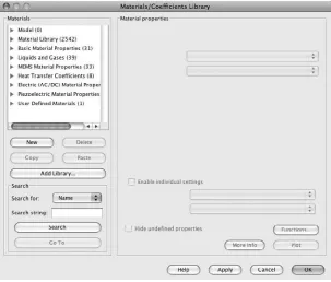
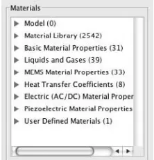
Materials and Database Guidelines and Considerations 39 COMSOL®Material Library Module: Searchable
Materials Library 40
MatWeb: Searchable Materials Properties Website 43 PKS-MPD: Searchable Materials Properties Database 48 References 61
Exercises 62
Chapter 3
1D Modeling 63
1D Guidelines for New COMSOL®Multiphysics®Modelers 63
1D Modeling Considerations 63 Coordinate System 64
iii
1D KdV Equation: Solitons and Optical Fibers 64 COMSOL KdV Equation Model 65
First Variation on the KdV Equation Model 77 Second Variation on the KdV Equation Model 83
1D KdV Equation Models: Summary and Conclusions 90 1D Telegraph Equation 90
COMSOL 1D Telegraph Equation Model 92 First Variation on the Telegraph Equation Model 98 Second Variation on the Telegraph Equation Model 105 1D Telegraph Equation Models: Summary
and Conclusions 110 References 112
Exercises 112
Chapter 4
2D Modeling 113
2D Guidelines for New COMSOL®Multiphysics®Modelers 113
2D Modeling Considerations 113 Coordinate System 114
2D Electrochemical Polishing (Electropolishing) Theory 115 COMSOL 2D Electrochemical Polishing Model 118
First Variation on the 2D Electrochemical Polishing Model 130 Second Variation on the 2D Electrochemical
Polishing Model 147
2D Electrochemical Polishing Models: Summary and Conclusions 165 2D Hall Effect Model Considerations 167
2D Hall Effect Model 171
First Variation on the 2D Hall Effect Model 186 Second Variation on the 2D Hall Effect Model 203 2D Hall Effect Models: Summary and Conclusions 221 References 222
Exercises 223
Chapter 5
2D Axisymmetric Modeling 225
2D Axisymmetric Guidelines for New COMSOL®
Multiphysics®Modelers 225
2D Axisymmetric Heat Conduction Modeling 229 2D Axisymmetric Cylinder Conduction Model 229 First Variation on the 2D Axisymmetric Cylinder
Conduction Model 240
Second Variation on the 2D Axisymmetric Cylinder Conduction Model, Including a Vacuum Cavity 250
2D Axisymmetric Cylinder Conduction Models: Summary and Conclusions 263
2D Axisymmetric Insulated Container Design 265 2D Axisymmetric Thermos_Container Model 265
First Variation on the 2D Axisymmetric Thermos_Container Model 285
Second Variation on the 2D Axisymmetric Thermos_Container Model 301
2D Axisymmetric Thermos_Container Models: Summary and Conclusions 316
References 318 Exercises 319
Chapter 6
2D Simple Mixed-Mode Modeling 321
2D Mixed-Mode Guidelines for New COMSOL®Multiphysics®
Modelers 321
2D Mixed-Mode Modeling Considerations 321 2D Coordinate System 322
2D Axisymmetric Coordinate System 324 Joule Heating and Heat Conduction Theory 324 Heat Conduction Theory 325
2D Resistive Heating Modeling 326 2D Resistive Heating Model 326
First Variation on the 2D Resistive Heating Model 345 Second Variation on the 2D Resistive Heating Model, Including
Alumina Isolation 366
2D Resistive Heating Models: Summary and Conclusions 388 2D Inductive Heating Considerations 389
2D Axisymmetric Coordinate System 389 2D Axisymmetric Inductive Heating Model 393 First Variation on the 2D Axisymmetric Inductive
Heating Model 411
Second Variation on the 2D Axisymmetric Inductive Heating Model 433
2D Axisymmetric Inductive Heating Models: Summary and Conclusions 453
References 457 Exercises 457
Chapter 7
2D Complex Mixed-Mode Modeling 459
2D Complex Mixed-Mode Guidelines for New COMSOL®
Multiphysics®Modelers 459
2D Complex Mixed-Mode Modeling Considerations 459 2D Coordinate System 461
Electrical Impedance Theory 461
2D Electric Impedance Sensor Model: Basic 464 Basic 2D Electric Impedance Sensor Model: Summary
and Conclusions 475
2D Electric Impedance Sensor Model: Advanced 477 2D Electric Impedance Sensor Models: Summary
and Conclusions 492
Generator and Power Distribution Basics 493 2D AC Generators: Static and Transient 498 2D AC Generator Model (2D_ACG_1): Static 498 2D AC Generator Model (2D_ACG_2): Transient 522 2D AC Generators, Static and Transient Models: Summary
and Conclusions 529
2D AC Generator: Sector—Static and Transient 530
2D AC Generator Sector Model (2D_ACGS_1): Static 531 2D AC Generators, Static Sector Model: Summary and
Conclusions 555
2D AC Generator Sector Model (2D_ACGS_2): Transient 557 2D AC Generators, Static and Transient Sector Models:
Summary and Conclusions 568 References 569
Exercises 570
Chapter 8
3D Modeling 571
3D Modeling Guidelines for New COMSOL®Multiphysics®
Modelers 571
Electrical Resistance Theory 573
Thin Layer Resistance Modeling Basics 575 3D Thin Layer Resistance Model: Thin Layer
Approximation 577
3D Thin Layer Resistance Model, Thin Layer Approximation: Summary and Conclusions 591
3D Thin Layer Resistance Model: Thin Layer Subdomain 593 3D Thin Layer Resistance Models: Summary
and Conclusions 608
Electrostatic Modeling Basics 611
3D Electrostatic Potential Between Two Cylinders 613 3D Electrostatic Potential Between Two Cylinders:
Summary and Conclusions 622
3D Electrostatic Potential Between Five Cylinders 622 3D Electrostatic Potential Between Five Cylinders: Summary
and Conclusions 633
Magnetostatic Modeling Basics 634
3D Magnetic Field of a Helmholtz Coil 636 3D Magnetic Field of a Helmholtz Coil: Summary
and Conclusions 649
3D Magnetic Field of a Helmholtz Coil with a Magnetic Test Object 652
3D Magnetic Field of a Helmholtz Coil with a Magnetic Test Object: Summary and Conclusions 666
References 669 Exercises 670
Chapter 9
Perfectly Matched Layer Models 671
Perfectly Matched Layer Modeling Guidelines and Coordinate Considerations 671 PML Theory 671
PML Models 676
2D Dielectric Lens Model, with PMLs 676 2D Dielectric Lens Model, with PMLs: Summary
and Conclusions 690
2D Dielectric Lens Model, without PMLs 691 2D Dielectric Lens Model, with and without PMLs:
Summary and Conclusions 702
2D Concave Mirror Model, with PMLs 707
2D Concave Mirror Model, with PMLs: Summary and Conclusions 723
2D Concave Mirror Model, without PMLs 724
2D Concave Mirror Model, with and without PMLs: Summary and Conclusions 736
References 744 Exercises 745
Chapter 10
Bioheat Models 747
Bioheat Modeling Guidelines and Coordinate Considerations 747 Bioheat Equation Theory 747
Tumor Laser Irradiation Theory 749
2D Axisymmetric Tumor Laser Irradiation Model 749 2D Axisymmetric Tumor Laser Irradiation Model: Summary
and Conclusions 768
Microwave Cancer Therapy Theory 769
2D Axisymmetric Microwave Cancer Therapy Model 770 2D Axisymmetric Microwave Cancer Therapy Model: Summary
and Conclusions 794 References 794
Exercises 795
The purpose of this book is to introduce hands-on model building and solving with COMSOL®Multiphysics® software to scientists, engineers, and others interested in
exploring the behavior of different physical device structures on a computer, before actually going to the workshop or laboratory and trying to build whatever it is.
The models presented in this text are built within the context of the physical world (applied physics) and are explored in light of first principles analysis techniques. As with any other method of problem solution, the information contained in the solutions from these computer simulations is as good as the materials coefficients and the fun-damental assumptions employed in building the models.
The primary advantage in combining computer simulation and first principles analysis is that the modeler can try as many different approaches to the solution of the same problem as needed to get it right (or at least close to right) in the workshop or laboratory the first time that device components are fabricated.
Acknowledgments
I would like to thank David Pallai of Jones and Bartlett Publishers for his ongoing encouragement in the completion of this book. I would also like to thank the many staff members of COMSOL, Inc., for their help and encouragement in completing this effort.
I would especially like to thank my wife, Beverly E. Pryor, for the many hours that she spent reading the manuscript and verifying the building instructions for each of the models. Any errors that remain are mine and mine alone.
Roger W. Pryor, Ph.D.
ix
x
COMSOL®Multiphysics®software is a powerful finite element (FEM), partial
dif-ferential equation (PDE) solution engine. The basic COMSOL Multiphysics soft-ware has eight add-on modules that expand the capabilities of the basic softsoft-ware into the following application areas: AC/DC, Acoustics, Chemical Engineering, Earth Science, Heat Transfer, MEMS, RF, and Structural Mechanics. The COMSOL Multiphysics software also has other supporting software, such as the CAD Import Module and the Material Library.
In this book, scientists, engineers, and others interested in exploring the behavior of different physical device structures through computer modeling are introduced to the techniques of hands-on building and solving models through the direct application of the COMSOL Multiphysics software, the AC/DC Module, the Heat Transfer Module, and the RF Module. Chapter 9 explores the use of perfectly matched layers (PML) in the RF Module. The final technical chapter (Chapter 10) explores the use of the bioheat equation in the Heat Transfer Module.
The models presented here are built within the context of the physical world (applied physics) and are presented in light of first principles analysis techniques. As with any other methodology of problem solution, the information derived from the modeling solutions through use of these computer simulations is only as good as the materials coefficients and the fundamental assumptions employed in building the models.
The primary advantage derived from combining computer simulation and first prin-ciples analysis is that the modeler can try as many different approaches to the solution of the same problem as needed to get it right (or at least close to right) in the workshop or laboratory before the first device components are fabricated and tested. The modeler can also use the physical device test results to modify the model parameters and arrive at a final solution more rapidly than by simply using the cut-and-try methodology.
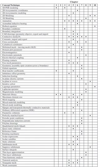
Chapter Topics
Concept/Technique 1 2 3 4 5 6 7 8 9 10
1D PDE modeling 2D Axisymmetric coordinates 2D Axisymmetric modeling 2D Modeling
3D Modeling Animation
Azimuthal inductive heating Bioheat equation Boundary conditions Boundary integration
CAD drawings (geometry objects), export and import Conductive media Pc
Constants, import and export Cross-section plot Cylindrical coordinates
Deformed mesh – moving mesh (ALE) Domain plot parameter
Electromagnetics Electrostatic potentials Electro-thermal coupling Floating contacts Free mesh parameters
Geometric assembly (pair creation across a boundary) Global equations
Heat transfer coefficients Imbalance-offset geometry Induction heating In-plane electric currents In-plane te waves Iterative solver Lagrange parameters Laplacian operator Magnetostatic modeling Materials library Maximum element size Mesh mapping Mixed-materials modeling Mixed-mode modeling
Opaque and transparent thermally conductive materials Ordinary differential equation (ODE)
Parametric solutions Perfectly matched layers Periodic point conditions Perpendicular induction currents Polyline drawings
Quadrilateral mesh (Quad) Quasi-static solutions Reference frame Rotating machinery Scalar expressions Scalar variables Static solutions Subdomain mesh Suppress subdomain Surface integrals Thin layer approximation Thin layer subdomain Time-harmonic analysis Transient analysis Triangular mesh Weak constraints
Chapter
FIGURE 1 COMSOL Concepts and Techniques
models in specific chapters are shown in Figure 2, and the physics concepts and tech-niques employed in the various models in specific chapters are shown in Figure 3.
These grids link the overall presentation of this book to the underlying modeling, mathematical, and physical concepts. In this book, in contrast to some other books with which the reader may be familiar, key ancillary information, in most cases, is contained in the notes.
Module Basic AC/DC Heat Transfer Materials Library Chapter
1 2 3 4 5 6 7 8 9 10
Please be sure to read, carefully consider, and apply, as needed, each note.
Chapter 1. Modeling Methodology
Chapter 1 begins the introduction to the modeling process by discussing the fundamental considerations involved: the hardware (computer platform), the coordinate systems (physics), the implicit assumptions (lower dimensionality considerations), and first prin-ciples analysis (physics). Three relatively simple 1D models are presented, built, and solved for comparison: one-pane, two-pane, and three-pane thermal insulation window structures. Comments are also included on common sources of modeling errors.
Chapter 2. Materials and Databases
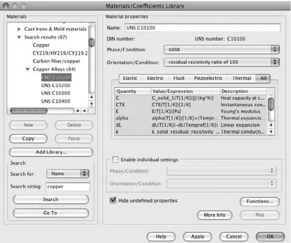
Chapter 2 briefly introduces three sources of materials properties data: the COMSOL Material Library, MatWeb, and the PKS-MPD.
The COMSOL Material Library is a module that can be added to the basic COM-SOL Multiphysics software package to expand the basic library that is already includ-ed. It contains data on approximately 2500 materials, including elements, minerals, soil, metal alloys, oxides, steels, thermal insulators, semiconductors, and optical mate-rials. Each material can have up to 27 defined properties. Each of those defined prop-erties is available as a function of temperature.
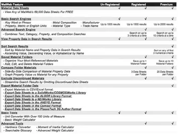
MatWeb is an online searchable subscription materials properties data source. MatWeb has three classes of access: Unregistered (free limited feature access), Registered Member (free expanded feature access), and Premium Member (fee-based
Introduction xiii
Physics Concepts 1
Chapter
2 3 4 5 6 7 8 9 10
AC induction
Anisotropic conductivity Antennas
Bioheat equation
Boltzmann thermodynamics Complex AC theory Complex impedance Concave mirror Coulomb gauge Dielectric lenses Distributed resistance Electrical impedance theory Electrochemical polishing
Electrostatic potentials in different geometric configurations Faraday’s law
First Estimate Review Foucault (eddy) currents Fourier’s law
Free-space permittivity Good first approximation Hall effect
Hard and soft nonlinear magnetic materials Heat conduction theory
Helmholtz coil Information transmission Insulated containers Joule heating Lorentz force Magnetic field Magnetic permeability Magnetic vector potential Magnetostatics
Maxwell’s equations
Mechanical to electrical energy conversion Microwave irradiation
Newton’s law of coding Ohm’s law
Optical (laser) irradiation Pennes’s equation
Perfectly matched layers: 2D planar, 3D cartesian cylindirical and Spherical
Perfusion Planck’s constant
Power transmission grids, AC and DC Power transmission, AC and DC Reactance
Semiconductor dual carrier types Skin depth
Soliton waves Telegraphs equation Thin layer resistance Vacuum
Vector dot product current (K*Nj_DC)
access to all features, plus selected data storage and modeling software formatted data export). MatWeb has 69,000 data sheets for materials, including plastics, metals, ceramics, semiconductors, fibers, and various other commercially available materials. PKS-MPD (Pryor Knowledge Systems—Materials Properties Database) is a new searchable materials properties database with data on more than 4000 materials, including elements, minerals, soil, metal alloys, oxides, steels, thermal insulators, semiconductors, optical materials, and biomaterials (tissue). Each material can have up to 43 defined properties. Each of those defined properties is associated with the temperature of measurement and the frequency of measurement. The collection of defined properties for each materials property datum is exportable in a format suitable for use with the COMSOL Multiphysics software.
Chapter 3. 1D Modeling
The first half of Chapter 3 models the 1D KdV equation and two variations. The KdV equation is a powerful tool that is used to model soliton wave propagation in diverse media (e.g., physical waves in liquids, electromagnetic waves in transparent media). It is easily and simply modeled with a 1D PDE mode model.
The second half of Chapter 3 models the 1D telegraph equation and two variations. The telegraph equation is a powerful tool that is used to model wave propagation in diverse transmission lines. It can be used to thoroughly characterize the propagation conditions of coaxial lines, twin pair lines, and microstrip lines, among other things. The telegraph equation is easily and simply modeled with a 1D PDE mode model.
Chapter 4. 2D Modeling
The first half of Chapter 4 models the 2D electrochemical polishing model. This model is a powerful tool that can be used to model surface smoothing for diverse proj-ects (e.g., microscope samples, precision metal parts, medical equipment and tools, large and small metal drums, thin analytical samples, vacuum chambers).
The second half of Chapter 4 models the 2D Hall effect. The 2D Hall Effect model is a powerful tool that can be used to model Hall effect magnetic sensors for sensing fluid flow, rotating and linear motion, proximity, current, pressure, and orientation.
Chapter 5. 2D Axisymmetric Modeling
The second half of Chapter 5 models three 2D axisymmetric thermos container models. From a comparison of the three models, it can be readily observed that the presence of a vacuum cavity significantly reduces the rate of heat flow through the model and the associated heat loss.
Chapter 6. 2D Simple Mixed-Mode Modeling
The first half of Chapter 6 models three 2D resistive heating models. These models are more illustrative of the mixed-mode modeling concept than they are directly amenable to the comparison of calculated values. They present different examples of the diversity of applied scientific and engineering model designs that can be explored using electro-thermal coupling and transient analysis. These models also demonstrate the significant power of relatively simple physical principles, such as Ohm’s law and Joule’s law.
The second half of Chapter 6 models three 2D axisymmetric inductive heating models. These models demonstrate the difference in level of complexity between single-coil and multi-coil models. In the Inductive_Heating_1 model, the concept of inductively produced heating is introduced. In the Inductive_Heating_2 model, the concept of inductively produced heating is applied to a practical application (a heated crucible) so as to present one example of the diverse applied scientific and engineering model designs that can be explored using electro-thermal coupling and transient analysis. In the Inductive_Heating_3 model, the crucible is filled with a commonly used metal for melting.
These models are examples of the good first approximation type of model. In other words, they demonstrate the significant power of relatively simple physical principles, such as Ohm’s law and Joule’s law, when applied in the COMSOL Multiphysics mod-eling environment. They could, of course, be modified by the addition of calculations, insulating materials, and heat loss through convection, among other changes.
Chapter 7. 2D Complex Mixed-Mode Modeling
The first third of Chapter 7 introduces two 2D electric impedance sensor models: basic and advanced. Those models employ high-frequency currents—1 MHz alternat-ing currents AC—to explore the differential impedance within a body of material in a noninvasive fashion. Such currents are applied to the material of the modeled body to locate volumes that differ in impedance from the impedance of the bulk material by monitoring the local impedance.
The basic version models the location of a fixed-volume impedance difference. The advanced version models the location of a fluctuating difference volume, as might be seen in a medical application measuring lung function. 2D electric impedance tomography research is currently exploring the application of this type of impedance
sensing measurement technology to the detection of breast cancer, lung function, brain function, and numerous other areas.
The second third of Chapter 7 introduces two 2D AC generator models: static and transient. These models generate low-frequency (60 Hz) current and voltage, as would be typically found on the power transmission grid. They demonstrate the use of both hard (not easily magnetized) and soft (easily magnetized) nonlinear magnetic materi-als in the construction of rotating machines for the conversion of mechanical energy to electrical energy.
The last third of Chapter 7 introduces two 2D AC generator sector models: static and transient. These models generate low-frequency (60 Hz) current and voltage, as would be typically found on the power transmission grid. They demonstrate the use of both hard (not easily magnetized) and soft (easily magnetized) nonlinear magnetic materials in the construction of a rotating machine for the conversion of mechanical energy to electrical energy. An ordinary differential equation (ODE) is incorporated into the sector model to handle the torque-related aspects of the model calculations.
Chapter 8. 3D Modeling
The first third of Chapter 8 models the 3D thin layer resistance model, thin layer approximation, and the thin layer resistance model, thin layer subdomain. The first model employs the thin layer approximation to solve a model by replacing the center domain with a contact-resistance identity pair. Such an approximation has broad appli-cability. It is important to note that the use of the thin layer approximation is applica-ble to any proapplica-blem in which flow is described by the divergence of a gradient flux (e.g., diffusion, heat conduction, flow through porous media under Darcy’s law).
The application of the thin layer approximation is especially valuable to the mod-eler when the differences in domain thickness are so great that the mesh generator fails to properly mesh the model or creates more elements than the modeling platform can handle (“run out of memory” problem). In those cases, this approximation may enable a model to be solved that would otherwise fail.
A direct comparison is made of the model solutions by comparing the results obtained from the cross-section plots. As seen from the examination of those plots, the only substantial difference between the two solutions is the electrical potential differ-ence across subdomain 2 (the thin layer). Thus the modeler can choose the imple-mentation that best suits his or her system and time constraint needs, without suffering excessive inaccuracies based on the approximation method.
Introduction xvii
tubes and particle accelerators to paint sprayers and dust precipitators). The 3D_ ESP_2 model is typical of those that might be found in a particle beam analyzer or a similar engineering or scientific device.
The last third of Chapter 8 models the 3D magnetic field of a Helmholtz coil. This model demonstrates the magnetic field uniformity of a Helmholtz coil pair. This mag-netostatic modeling technique can be applied to a diverse collection of scientific and engineering applications (e.g., ranging from magnetometers and Hall effect sensors to biomagnetic and medical studies).
A related model, the 3D magnetic field of a Helmholtz coil with a magnetic test object, demonstrates the magnetic field concentration when a high relative permeabil-ity object lies within the field of the Helmholtz coil. This magnetostatic modeling technique can be applied to a diverse collection of scientific and engineering test, measurement, and design applications.
Chapter 9. Perfectly Matched Layer Models
The first half of Chapter 9 introduces the 2D dielectric lens models, with and with-out perfectly matched layers (PMLs). [The PML model best approximates a free space environment (no reflections).] Comparison is made between the two models. The differences in the electric field, z-component visualizations between the PML and no-PML models amount to approximately 2%. Depending on the nature of the problem, such differences may or may not be significant. What these differences show the modeler is that he or she needs to understand the application environment well so as to build the best model. For other than free space environments, the mod-eler needs to determine the best boundary condition approximation using standard practices and a first principles approach. Always do a first principles analysis of the environment before building the model.
The second half of Chapter 9 introduces the 2D concave mirror models, with and without PMLs. There are only small differences in the electric field, z-component visualizations between the PML and no-PML models for the concave mirror. This lack of large differences between the PML and no-PML models again shows the modeler that he or she needs to understand the relative importance of the modeled values to evaluate the application and the application environment so as to build the best model.
Chapter 10. Bioheat Models
The results (estimated time values) from the model calculations will significantly reduce the effort needed to determine an accurate experimental value. The guiding principle needs to be that tumor cells die at elevated temperatures. The literature cites temperatures that range from 42 °C (315.15 K) to 60 °C (333.15 K).
The first half of Chapter 10 models the bioheat equation as applied with a pho-tonic heat source (laser). The second half of the chapter models the bioheat equation as applied with a microwave heat source.
1
Modeling Methodology
1
In This Chapter
Guidelines for New COMSOL®Multiphysics®Modelers
Hardware Considerations Coordinate Systems Implicit Assumptions
1D Window Panes Heat Flow Models 1D Single-Pane Heat Flow Model 1D Dual-Pane Heat Flow Model 1D Triple-Pane Heat Flow Model First Principles Applied to Model Definition Common Sources of Modeling Errors
Guidelines for New COMSOL
®Multiphysics
®Modelers
Hardware Considerations
There are two basic rules to selecting hardware that will support successful modeling. First, new modelers should be sure to determine the minimum system requirements that their version of COMSOL®Multiphysics® software needs before borrowing or
buying a computer to run their new modeling software. Second, these new modelers should run their copy of COMSOL Multiphysics software on the best platform with the highest processor speed and the most memory obtainable: The bigger and faster, the better. It is the general rule that the speed of model processing increases directly as a function of the processor speed, the number of platform cores, and the available memory.
The number of platform cores is equal to the number of coprocessors designed into the computer (e.g., one, two, four, eight, . . .).
The platform that this author uses is an Apple®Mac Pro®, running Mac OS X®
This Mac Pro has four 3 GHz cores and 16 GB of RAM. This platform, as configured, is more powerful, more versatile, more stable, and more cost-effective than other poten-tial choices. It can handle complex 3D models in short computational times (more speed, more memory)—that is, in minutes instead of the hours that may be required by less powerful systems. This configuration can run any of the 32-bit COMSOL Multiphysics software, when using COMSOL Multiphysics Version 3.4. The Apple hardware is con-figured for 64-bit processing and will run at the 64-bit rate when using COMSOL Multiphysics Version 3.5. If new modelers desire a different 64-bit operating system than Macintosh OS X, then they will need to choose either a Sun®or a Linux®platform,
using UNIX©or a PC with a 64-bit Microsoft Windows operating system.
The “3 GHz” specification is the operating speed of each of the cores and the “16 GB” is the total shared random access memory (RAM). The “64-bit” refers to the width of a processor instruction.
Once the best available processor is obtained, within the constraints of your budg-et, install your copy of COMSOL Multiphysics software, following the installer instructions. Once installed, COMSOL Multiphysics software presents the modeler with a graphical user interface (GUI). For computer users not familiar with the GUI concept, information in such an interface is presented primarily in the form of pictures with supplemental text, not exclusively text.
Coordinate Systems
Figure 1.1 shows the default (x-y-z) coordinate orientation for COMSOL modeling calculations. This coordinate system is based on the right-hand rule.
The right-hand rule is summarized by its name. Look at your right hand, point the thumb up; point your first finger away from your body, at a right angle (90 degrees) to your thumb; and point your second finger at a right angle to the thumb and first finger, parallel to your body. Your thumb represents the z-axis, your first finger represents the x-axis, and your second finger represents the y-axis.
In this right-handed coordinate system, xrotates into yand generates z. If you have a need to convert your model from the x-y-zframe to a Spherical Coordinate frame, then the transformation can be implemented using built-in COMSOL mathematical functions. The x-y-z to spherical coordinate conversion is achieved through the following equations:
x-yplane rotational angle (phi): (1.2)
x-zplane rotational angle (theta): (1.3)
The built-in function sqrt(argument) indicates that COMSOL Multiphysics will take the positive square root of the argument contained between the parentheses. The built-in function a tan2(argument) indicates that COMSOL Multiphysics will convert the argument contained between the parentheses to an angle in radians (in this case, phi). The built-in function a cos(argument) indicates that COMSOL Multiphysics will convert the argument contained between the parentheses to an angle in radians (in this case, theta).
To employ these spherical conversion equations in your model, you will need to start COMSOL Multiphysics, select “3D” in the Model Navigator Screen, select the desired Application Mode, and click the OK button. Using the pull-down menu, select Options > Expressions > Scalar Expressions and then enter equations 1.1, 1.2, and 1.3 in the Scalar Expressions window, as shown in Figure 1.2.
theta5a cos1z
/
r2u
phi5a tan21y, x2
f
Guidelines for New COMSOL Multiphysics Modelers 3
B1 B2 B3 y z x –1 –0.5 0.5 1 –1 –0.5 0 0.5 1 –1 –0.5 0 0.5 1 0
When a list of operations is presented sequentially (A > B > C > D), the modeler is expected to execute those operations in that sequence in COMSOL.
Once these equations are available in the model, the x-y-zcoordinates can be con-verted as shown in Figures 1.3 and 1.4.
The rotational sense of an angular transform is determined by viewing the angular rotation as one would view a typical analog clock face. The vector rrotating from xinto yfor a positive angle phi is counterclockwise, because phi equals zero at the positive x-axis. The vector r rotating from z into x for a positive angle theta is clockwise, because theta equals zero at the positive z-axis.
FIGURE 1.2 COMSOL Multiphysics 3D Scalar Expressions window with the spherical coordinate transform equations entered
FIGURE 1.3 Spherical coordinate transform angle and rotational sense for ( ) phif phi
x
y
z
As all potential COMSOL modelers know, the Cartesian (x-y-z) and Spherical Coordinate (r-phi-theta) reference frames are not the only coordinate systems that can be used as the basis frame for Multiphysics models. In fact, when you first open the Model Navigator, you are given the option and are required to choose one of the following mod-eling coordinate systems: 1D, 2D, 3D, Axial Symmetry (1D), or Axial Symmetry (2D). The coordinate system that you choose determines the geometry and specific subgroup of COMSOL Application Modes that can be applied in that selected geometry (geometries).
An Application Mode is the initial collection of equations, independent variable(s), dependent variable(s), default settings, boundary conditions, and other properties that are appropriate for the solution of problems in that branch of physics (e.g., acoustics, electromagnetics, heat transfer). As indicated by the name “Multiphysics,” multiple branches of physics can be applied within each model. Diverse models that demonstrate the application of the multiphysics concept will be explored in detail as this book progresses.
Implicit Assumptions
A modeler can generate a first-cut problem solution as a reasonable estimate, by choosing initially to use a lower-dimensionality coordinate space than 3D (e.g., 1D, 2D Axisymmetric). By making a low-dimensionality geometric choice, a modeler can significantly reduce the total time needed to achieve a detailed final solution for the chosen prototype model. Both new modelers and experienced modelers alike must be especially careful to fully understand the underlying (implicit) assumptions, unspeci-fied conditions, and default values that are incorporated into the model as a result of simply selecting the lower-dimensionality geometry.
Guidelines for New COMSOL Multiphysics Modelers 5
FIGURE 1.4 Spherical coordinate transform angle and rotational sense for ( ) thetau
z
x r
y
A first-cut solution is the equivalent of a back-of-the-envelope or on-a-napkin solution. Solutions of this type are relatively easy to formulate, are quickly built, and provide a first estimate of whether the final solution of the full problem is deemed to be (should be) within reasonable bounds. Creating a first-cut solution will often allow the modeler to decide whether it is worth the time and money required to create a fully implemented higher-dimensionality (3D) model.
Space, as all modelers know, comes with four basic dimensions: three space dimensions (x-y-z) and one time dimension (t). For example, the four dimensions might be x-y-z-t, orr- - -t. Relativistic effects can typically be neglected, except in cases of high velocity or ultra-high accuracy. Neither of these types of problems will be covered in this book.
Relativistic effects typically become a concern only for bodies in motion with a velocity approaching that of the speed of light (~3.0 108 m/s) or for ultra-high resolution time calculations at somewhat lower velocities.
The types of calculations presented within this book are typically for steady-state models or for relatively low-velocity transient model solutions. Any transient solution model can be solved using a quasi-static methodology.
In a steady-state model, the controlling parameters are defined as numerical constants and the model is allowed to converge at the equilibrium state defined by the specified constants. In the quasi-static methodology, a model solution to a problem is found by initially treating the model as a steady-state problem. Incrementally modifying the modeling constants then moves the model problem solution toward the desired transient solution.
1D Window Panes Heat Flow Models
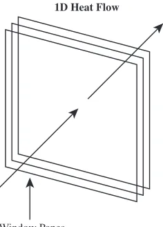
Consider, for example, a brief comparison between a relatively simple 1D heat flow model and the identical problem presented as a 3D model. The models considered here are those of a single-pane, dual-pane, or triple-pane window mounted in the wall of a building on a typical winter’s day. The questions to be answered are Why use a dual-pane window? and Why use a triple-dual-pane window?
1D Single-Pane Heat Flow Model
Run the COMSOL Multiphysics application. Select “New” and then select “1D” in the Model Navigator. Then select “COMSOL Multiphysics.” Select “Heat Transfer” followed by “Conduction” and then “Steady-state analysis.” Click OK.
3 u
After the 1D workspace appears, enter the constant values needed for this model: Use the menu bar to select Options > Constants. Enter the following items: T_in tab 70[degF] tab Interior Temperature tab T_out tab 0[degF] tab Exterior Temperature tab p tab 1[atm] (in Version 3.4) or 1.01325e5[Pa] (for earlier versions) tab air pressure tab; see Figure 1.5. Click the Apply button. These entries in the Constants window define the Interior Temperature, the Exterior Temperature, and the air pressure for use in this model. Click on the disk icon in the lower-left corner of the Constants window (Export Variables to File) to save these constants as ModelOC_1D_WP1.txt for use in the comparison models to follow later in this chapter. Click the OK button.
Next, draw a line to represent the thickness of a 1D window pane: Use the menu bar and select Draw > Specify Objects > Line. Enter the following: 0.000 space 0.005; see Figure 1.6. Leave the default Polyline, and click the OK button. Click the Zoom Extents icon in the toolbar.
Once the Zoom Extents icon is clicked, the specified 0.005 m line will appear in the workspace, as shown in Figure 1.7.
After the 0.005 m line has been created in the workspace, use the menu bar and select Physics > Subdomain Settings > 1. The window shown in Figure 1.8 contains the known properties of copper (Cu) as the default materials properties values.
1D Window Panes Heat Flow Models 7
FIGURE 1.5 1D Constants specification window
If copper is not the material of choice, as in this heat transfer model, then the materials property values need to be changed.
The implicit assumption here would be that the default values in the Subdomain Settings window are the correct values that the modeler needs to build the desired model. Specifically, that assumption would be true only if the modeler were building the heat transfer model using copper. In general, that implicit assumption is not correct. The modeler needs to know before building any new models what the approximate expected values are for the particular properties of the materials selected for use in the model. A number of sources have detailed materials properties values available: Some sources are available at no cost, while other sources have different levels of availability for different fees. Materials properties sources are discussed in Chapter 2.
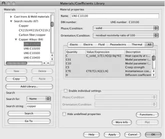
For this model, click the Load button, and then select “Basic Materials Properties” and “Silica Glass.” Click OK. All the appropriate values displayed in the Value/ Expression subwindows in the Subdomain Settings window are altered as the new val-ues are loaded from the library. (Silica glass has a thermal conductivity value rough-ly 0.35% of that of copper.)
Once the thermal conductivity is loaded from the materials properties library, enter T_in in the Textand Tambtranswindows, as shown in Figure 1.9.
Click the Init button and enter T_in as shown in Figure 1.10. Click OK. Setting the T_in value as the initial temperature of the window pane (subdomain 1) allows for quicker convergence of the model and avoids any singularities.
1D Window Panes Heat Flow Models 9
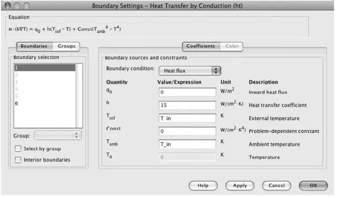
Now the modeler needs to enter the appropriate Boundary Settings. Using the menu bar, select Physics > Boundary Settings. After the Boundary Settings window appears, as shown in Figure 1.11, select “1” in the Boundary Settings Boundary selec-tion window.
FIGURE 1.11 Boundary Settings window
Next, select “Heat flux” from the Boundary conditions pull-down menu. Enter 15 in the Heat transfer coefficient window (h). Enter T_in in the External temper-ature window (Tinf). Enter T_in in the Ambient temperature window (Tamb). Click the Apply button. Figure 1.12 shows the filled-in Boundary Settings window for boundary 1.
Now select “2” in the Boundary Settings Boundary selection window. Select “Heat flux” as the Boundary condition. Enter 15 in the Heat transfer coefficient win-dow (h). Enter T_out in the External temperature winwin-dow (Tinf). Enter T_out in the Ambient temperature window (Tamb). Click the Apply button. Figure 1.13 shows the filled-in Boundary Settings window for boundary 2. Click OK.
All the Subdomain Settings and the Boundary Settings have now been either cho-sen or entered. The next step is to mesh the model. In this simple model, all the mod-eler needs to do is use the toolbar and select “Initialize Mesh.” Figure 1.14 shows the initial mesh. The line segments between the dots are the mesh elements.
To improve the resolution, the mesh will be refined twice. All the modeler needs to do is use the toolbar and select Refine Mesh > Refine Mesh. The refined mesh of the single-pane model now contains the 60 elements shown in Figure 1.15, rather than the original 15 elements shown in Figure 1.14.
For this model, the software will be allowed to automatically select the Solver and Solver Parameters. To solve this model, go to the menu bar and select Solve > Solve Problem. The solution is found almost immediately, in 0.014 second. The solution is plotted using the default Postprocessing values and is shown in Figure 1.16.
1D Window Panes Heat Flow Models 11
The precise length of time required for the solution of a given model depends directly on the configuration of the platform and the overhead imposed by the operating system.
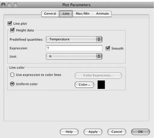
The implicit assumption here would be that the default values in the Postprocessing window are the correct values that the modeler needs to plot the calculated results of the built model. Specifically, that assumption in general will not be true. For example, in the case of this model, the default plot is in Kelvins (K), when the modeler would probably prefer degrees Fahrenheit. Also, it would be helpful to show the change in temperature as a function of the distance into the window pane.
The modeler needs to know before building a new model what the approximate expected resultant values are for the particular properties of the materials selected for use in the model. A firm understanding of the basic physics involved and the appropriate conservation laws that apply to the model are required for analysis, understanding, and configuration of the Postprocessing presentation(s).
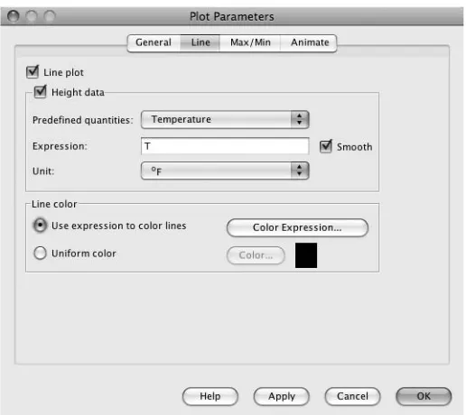
The plot presentation is changed as follows: Select Postprocessing > Plot Parameters from the menu bar. When the Plot Parameters window shown in Figure 1.17 appears, select “Line” (Figure 1.18) and then “°F(degF)” from the Unit pull-down bar.
Select “Use expression to color line.” Click the Color Expression button to display the Line Color Expression window (Figure 1.19). Select “ (degF)” from the Unit pull-down bar. Click OK, and then click OK again. The Plot Presentation will be rendered as shown in Figure 1.20.
1D Single-Pane Analysis and Conclusions
The 1D single-pane window model, though simple, reveals several fundamental factors about the physics of heat flow through the single-pane window. The interior tempera-ture T_in was established at 70 . The exterior temperature T_out was established at 0 °F. The calculated temperature at the midpoint of the single pane is the median value
°F
°F
of the interior and exterior temperatures, 35 . The temperature difference between the inner surface of the pane and the outer surface of the pane is approximately 2 .
The temperature difference between the air in the heated room (70 ) and the interior surface of the single pane (35.9 ) is approximately 34 . This temperature difference between the ambient temperature and the single-pane window will at least result in water vapor condensation (fogging) and heat loss to the exterior.
When building models, be sure to save early and often. °F °F
°F °F °F
1D Window Panes Heat Flow Models 15
FIGURE 1.18 1D single-pane Plot Parameters Line window
1D Dual-Pane Heat Flow Model
This 1D model explores the physics of a dual-pane window with an air space between the panes. This model is parametrically similar to the single-pane window model for ease of comparison of the modeling results.
Run the COMSOL Multiphysics application. Select “New” and then select “1D” in the Model Navigator. Select COMSOL Multiphysics > Heat Transfer > Conduction > Steady-state analysis. Click OK.
After the 1D workspace appears, use the menu bar to select Options > Constants. Import the file ModelOC_1D_WP1.txt saved earlier. To import this file, click on the Folder icon in the lower-left corner of the Constants window. These imported entries, as shown in Figure 1.21, define the Interior Temperature, the Exterior Temperature, and the air pressure for use in this model and the models to follow.
button. Finally, using the menu bar, draw the third line. Select Draw > Specify Objects > Line. Enter 0.015 space 0.020 in the window. Leave the default Polyline, and click the OK button. Figure 1.24 shows the results of the model line creation before click-ing the Zoom Extents icon in the toolbar.
Once the Zoom Extents icon is clicked, the specified dual-pane Window model will appear in the workspace as shown in Figure 1.25.
Next, using the menu bar, select Physics > Subdomain Settings. Once the Subdomain Settings window appears, select “1” in the Subdomain selection window. For this model, select Load > Basic Materials Properties > Silica Glass. Click OK. All the appropriate values displayed in the Value/Expression subwindows in the Subdomain Settings window are altered as the new values are loaded from the library. (Silica glass has a thermal conductivity value roughly 0.35% of that of copper.)
Once the thermal conductivity is loaded from the materials properties library, enter T_in in the Textand Tambtranswindows, as shown in Figure 1.26. Click the Apply button. Next, select “2” in the Subdomain selection window. For this model, select Load > Basic Materials Properties > Air, 1 atm. Click OK. All the appropriate values dis-played in the Value/Expression subwindows in the Subdomain Settings window are altered as the new values are loaded from the library.
1D Window Panes Heat Flow Models 17
FIGURE 1.21 1D dual-pane Constants specification window
Once the thermal conductivity is loaded from the materials properties library, enter T_in in the Textand Tambtranswindows, as shown in Figure 1.27. Click the Apply button. Next, select “3” in the Subdomain selection window. For this model, Select Library materials list > Silica Glass. The previously selected values loaded from the materials library are loaded into this subdomain.
Once the thermal conductivity is loaded from the materials properties library, enter T_out in the Textand Tambtranswindows, as shown in Figure 1.28. Click the Apply button. Next, set the initial conditions for each subdomain (1, 2, 3) by clicking the Init button and then entering the initial conditions shown in Table 1.1. Click OK.
Now, the modeler needs to enter the appropriate Boundary Settings. Using the menu bar, select Physics > Boundary Settings, as shown in Figure 1.29.
Once the Boundary Settings window appears, select “1” in the Boundary selec-tion window. Select “Heat flux” as the Boundary condiselec-tion. Enter 15 in the Heat transfer coefficient window (h). Enter T_in in the External temperature window (Tinf). Enter T_in in the Ambient temperature window (Tamb). Click the Apply button. Figure 1.30 shows the filled-in Boundary Settings window for boundary 1.
1D Window Panes Heat Flow Models 19
Subdomain 1 2 3
Init T_in T_in T_out
Table 1.1 Subdomain Settings, Initial Conditions
FIGURE 1.27 1D dual-pane Subdomain Settings Physics window settings, air gap
Now select “4” in the Boundary Settings Boundary selection window. Select “Heat flux” as the Boundary condition. Enter 15 in the Heat transfer coefficient win-dow (h). Enter T_out in the External temperature winwin-dow (Tinf). Enter T_out in the Ambient temperature window (Tamb). Click the Apply button. Figure 1.31 shows the filled-in Boundary Settings window for boundary 4. Click OK.
1D Window Panes Heat Flow Models 21
FIGURE 1.29 1D dual-pane Boundary Settings window
At this point, a new modeler probably wonders why no conditions have been specified for boundaries 2 and 3. The COMSOL Multiphysics software default condition is to automatically establish continuity for interior boundaries. The numbers for boundaries 2 and 3 are grayed out to indicate that they are not available for setting. The default boundary settings can be overridden, if needed, by the advanced modeler by clicking the Interior boundaries check box to make boundaries 2 and 3 accessible.
Once all the Subdomain Settings and the Boundary Settings for this model have been either chosen or entered, the next step is to mesh the model. In this simple model, all the modeler needs to do is use the menu bar and Select “Initialize Mesh.” Figure 1.32 shows the initial mesh with 16 elements.
The mesh will be refined twice to improve the resolution. All the modeler needs to do is use the toolbar and select Refine Mesh > Refine Mesh. The refined mesh of the dual-pane model now contains the 64 elements shown in Figure 1.33, rather than the original 16 elements shown in Figure 1.32.
For this model, the software will be allowed to automatically select the Solver and Solver Parameters. To solve this model, go to the menu bar and select Solve > Solve Problem. The solution is found almost immediately, in 0.317 second (the time to solu-tion will vary, depending on the platform). The solusolu-tion is plotted using the default Postprocessing values and is shown in Figure 1.34.
The implicit assumption here would be that the default values in the Postprocessing window are the correct values that the modeler needs to plot the calculated results of the built model. Specifically, that assumption in general will not be true. The modeler needs to know before building a new model what the approximate expected resultant values are for the particular properties of the materials selected for use in the model. A firm understanding of the basic physics involved and the appropriate conservation laws that apply to the model are required for analysis, understanding, and configuration of the Postprocessing presentation(s).
The plot presentation is changed as follows: Select Postprocessing > Plot Parameters from the menu bar. When the Plot Parameters window shown in Figure 1.35 appears, select “Line” (Figure 1.36) and then “ (degF)” from the Unit pull-down bar (Figure 1.37). Select “Use expression to color lines.” Click the Color Expression button
°F
1D Window Panes Heat Flow Models 23
FIGURE 1.32 1D dual-pane window with air gap with initialized mesh
1D Window Panes Heat Flow Models 25
FIGURE 1.36 1D dual-pane Plot Parameters Line window
FIGURE 1.39 1D single-pane window solution set to use °F
(Figure 1.38). Select “ (degF)” from the Unit pull-down bar (Figure 1.39). Click OK, and then click OK again. The plot presentation will be rendered as shown in Figure 1.40.
Dual-Pane Analysis and Conclusions
The 1D dual-pane window model, though simple, reveals several fundamental factors about the physics of heat flow through the dual-pane window. The interior tempera-ture T_in was established at 70 , as in the single-pane model. The exterior temper-ature T_out was established at 0 , as in the single-pane model. The calculated temperature at the midpoint of the single pane is the median value of the interior and
°F °F °F
exterior temperatures, 35 . The temperature difference between the inner surface of the left pane and the outer surface of the left pane is approximately 0.48 . The temperature difference between the inner surface of the right pane and the outer sur-face of the right pane is also approximately 0.48 . The temperature difference between the inner surface and the outer surface of the dual-pane window is approxi-mately 53 , as compared to approximately 2 for the single-pane window.
The temperature difference between the air in the heated room (70 ) and the interior surface (61.5 ) of the dual-pane window is approximately 8.5 . This small temperature difference will result in some heat loss and minimal water vapor condensation (fogging).
Compare the result for the dual-pane window to that of the single-pane window. The temperature difference between the air in the heated room (70 ) and the interi-or surface of the single-pane window (35.9 ) is approximately 34 . This temper-ature difference between the ambient tempertemper-ature and the single-pane window will at least result in water vapor condensation (fogging) and heat loss to the exterior.
1D Triple-Pane Heat Flow Model
This 1D model explores the physics of a triple-pane window with an air space between each pair of panes. This model is parametrically similar to the single-pane and dual-pane models for ease of comparison of the modeling results.
°F °F °F °F °F °F °F °F °F °F °F
Line Start End
1 0.000 0.005
2 0.005 0.015
3 0.015 0.020
4 0.020 0.030
5 0.030 0.035
Table 1.2 Triple-Pane Window Workspace Lines
Run the COMSOL Multiphysics application. Select “New” and then “1D” in the Model Navigator. Select COMSOL Multiphysics > Heat Transfer > Conduction > Steady-state analysis. Click the OK button.
After the 1D workspace appears, use the menu bar to select Options > Constants. Import the file ModelOC_1D_WP1.txt saved earlier. To import this file, click on the Folder icon in the lower-left corner of the Constants window. These imported entries, as shown in Figure 1.41, define the Interior Temperature, the Exterior Temperature, and the air pressure for use in this model and the models to follow.
Modeling a triple-pane window requires that five lines be drawn in the workspace window. The drawn lines represent the left (first) pane, the first air space, the center (second) pane, the second air space, and the right (third) pane, respectively. Use the toolbar to draw the first line: Select Draw > Specify Objects > Line. Enter 0.000 space 0.005 in the window. Leave the default Polyline, and then click the OK button. Next, use the menu bar to draw the remaining four lines, as indicated in Table 1.2. Then, click the Zoom Extents icon in the toolbar. The finished workspace configuration is shown in Figure 1.42.
Next, using the menu bar, select Physics > Subdomain Settings. Once the Subdomain Settings window appears, select “1” in the Subdomain selection window. For this model, select Load > Basic Materials Properties > Silica Glass. Click OK (see Figure 1.43). Enter the remaining Subdomain Settings as shown in Table 1.3.
1D Window Panes Heat Flow Models 31
FIGURE 1.45 Blank 1D triple-pane Boundary Settings window
Once the Boundary Settings window appears, select “1” in the Boundary selec-tion window. Select “Heat flux” as the Boundary condiselec-tion. Enter 15 in the Heat transfer coefficient window (h). Enter T_in in the Ambient temperature window (Tinf). Enter T_in in the External temperature window (Tamb). Click the Apply button. Figure 1.46 shows the filled-in Boundary Settings window for boundary 1. Fill in the
remaining Boundary Settings as shown in Table 1.5. Click the Apply button after each entry, and click OK at the end of the process.
At this point, as mentioned in the discussion of the dual-pane window model, no conditions are specified for boundaries 2, 3, 4, and 5, because the COMSOL Multiphysics software default condition is to automatically establish continuity for interior boundaries. The numbers for boundaries 2, 3, 4, and 5 are grayed out to indicate that they are not available for setting. The default boundary settings can be overridden, if needed, by the advanced modeler.
Once all the Subdomain Settings and the Boundary Settings for this model have been either chosen or entered, the next step is to mesh the model. In this model, all the modeler needs to do is use the toolbar and select “Initialize Mesh.” Figure 1.47 shows the initial mesh with 16 elements.
For this model, the software will be allowed to automatically select the Solver and Solver Parameters. To solve this model, go to the menu bar and select Solve > Solve Problem. The solution is found almost immediately, in 0.346 second (the length of time to solution will vary depending on the platform). The solution is plotted using the default Postprocessing values and is shown in Figure 1.49.
As noted earlier in the solutions of the single-pane and dual-pane models, the postprocessing parameters need to be altered to reveal the most information at a glance.
The plot presentation is changed as follows: Select Postprocessing > Plot Parameters from the menu bar. When the Plot Parameters window appears, select “Line” and then “ (degF)” from the Unit pull-down bar. Select “Use expression to color lines.” Click the Color Expression button. Select “ (degF)” from the Unit pull-down bar. Click OK and then click OK again. The plot presentation will be rendered as shown in Figure 1.50.
Triple-Pane Analysis and Conclusions
The 1D triple-pane window model reveals several fundamental factors about the physics of heat flow through the triple-pane window. The interior temperature T_in was established at 70 , as in the single-pane and dual-pane models. The exterior temperature T_out was established at 0 , as in the single-pane and dual-pane models. The temperature difference between the inner surface and the outer surface of the three different window types are compared as shown in Table 1.6.
The temperature difference between the air in the heated room (70 ) and the interior surface of the triple-pane window (65.2 °F) is approximately 4.8 °F. This
°F °F
°F
minimal temperature difference will result in little heat loss and little, if any, water vapor condensation (fogging).
Comparing the results for the three different window configuration models shows that there will be a large reduction in heat loss and annoyance factors (con-densation) associated with a change from a single-pane window to a dual-pane win-dow design. The incremental cost of such a design change would typically be less than 100%. However, adding the third pane to the window design reduces the heat loss by only a few percentage points and adds little to the cosmetic enhancement of the design (lack of fogging).
One of the basic reasons for modeling potential products is to evaluate their relative performance before the actual building of a first experimental physical model. Comparison of these three window models allows such a comparison to easily be made on a “first principles” basis, which will be discussed in the following section of this chapter. That approach is known as the “Model first, build second” approach to engineering design. When the model properly incorporates the fundamental materials properties and design factors, both the time and the cost to develop a fully functional prototype product are significantly reduced.
First Principles Applied to Model Definition
First principles analysis is an analysis whose basis is intimately tied to the funda-mental laws of nature. In the case of models described in this book, the modeler should be able to demonstrate both to himself or herself and to others that the calcu-lated results derived from those models are consistent with the laws of physics and the observed properties of materials. Basically, the laws of physics require that what goes in (e.g., as mass, energy, charge) must come out (e.g., as mass, energy, charge) or must accumulate within the boundaries of the model.
First Principles Applied to Model Definition 35
Single Dual Triple
T 2 53 60
across all panes
T 34 8.5 4.8
inner pane surface
to room ambient temperature
1°F2: D
1°F2: D
In the COMSOL Multiphysics software, the default interior boundary conditions are set to apply the conditions of continuity in the absence of sources (e.g., heat generation, charge generation, molecule generation) or sinks (e.g., heat loss, charge recombination, molecule loss).
The careful modeler will be able to determine by inspection that the appropriate factors have been considered in the development of the specifications for the various geometries, for the material properties of each subdomain, and for the boundary con-ditions. He or she must also be knowledgeable of the implicit assumptions and default specifications that are normally incorporated into the COMSOL Multiphysics soft-ware model, when a model is built using the default settings.
Consider, for example, the three window models developed earlier in this chapter. By choosing to develop those models in the simplest 1D geometrical mode, the implicit assumption was made that the heat flow occurred in only one direction. That direction was basically normal to the surface of the window and from the high tem-perature (inside temtem-perature) to the low temtem-perature (outside temtem-perature), as shown by the heat flow indicator in Figure 1.51.
That assumption essentially eliminates the consideration of heat flow along other paths, such as through the window frame, through air leaks around the panes, and so forth. It also assumes that the materials are homogeneous and isotropic, and that there are no thin thermal barriers at the surfaces of the panes. None of these assumptions is typically true in the general case. However, by making such assumptions, it is possi-ble to easily build a first approximation model.
Window Panes
1D Heat Flow
A first approximation model captures all of the essential features of the problem that needs to be solved, without dwelling excessively on minutiae. A good first approximation model will yield an answer that is sufficiently accurate to enable the modeler to determine whether he or she needs to invest the time and resources necessary to build a higher-dimensionality, significantly more-accurate model.
Common Sources of Modeling Errors
There are four primary sources of modeling errors: insufficient model preparation time, insufficient attention to detail during the model preparation and creation phase, insufficient understanding of the physical and modeling principles required for the creation of an adequate model, and lack of a comprehensive understanding of what defines an adequate model in the modeler’s context. The most common modeling errors are those that result from the modeler taking insufficient care in either the devel-opment of model details or the incorporation of conceptual errors and/or the genera-tion of keying errors during data/parameter/formula entry.
One primary source of errors occurs during the process of naming variables. The modeler should be careful to never give the same name to his or her variables as COMSOL gives to the default variables. COMSOL Multiphysics software seeks a value for the designated variable everywhere within its operating domain. If two or more variables have the same designation, an error is created. Also, it is best to avoid human errors by using uniquely distinguishable characters in variable names (i.e., avoid using the lowercase “L,” the number “1,” and the uppercase “I,” which in some fonts are relatively indistinguishable; similarly, avoid the uppercase “O” and the number zero “0”). Give your variables meaningful names (e.g., T_in, T_out, T_hot). Also, variable names are case sensitive; that is, T_in is not the same as T_IN.
The first rule in model development is to define the nature of the problem to be solved and to specify in detail which aspects of the problem the model will address. The definition of the nature of the problem should include a hierarchical list of the magnitude of the relative contribution of physical properties vital to the functioning of the anticipated model and their relative degree of interaction.
Examples of typical physical properties that are probably coupled in any developed model are heat and geometrical expansion/contraction (liquid, gas, solid), current flow and heat generation/reduction, phase change and geometrical expansion/ contraction (liquid, gas, solid) and/or heat generation/reduction, and chemical reactions. Be sure to investigate your problem and build your model carefully.
Having built the hierarchical list, the modeler should then estimate the best phys-ical, least-coupled, lowest-dimensionality modeling approach to achieve the most meaningful first approximation model.
Exercises
1. Build, mesh, and solve the 1D single-pane window problem presented earlier in this chapter.
2. Build, mesh, and solve the 1D dual-pane window problem presented earlier in this chapter.
3. Build, mesh, and solve the 1D triple-pane window problem presented earlier in this chapter.
39
Materials and Databases
2
In This Chapter
Materials and Database Guidelines and Considerations
COMSOL®Material Library Module: Searchable Materials Library
MatWeb: Searchable Materials Properties Website PKS-MPD: Searchable Materials Properties Database
Materials and Database Guidelines and Considerations
Materials selection and definition are the most important tasks performed by the mod-eler during the preliminary stages of model building preparation. The selection of appropriate materials is vital to the ultimate functionality of the device or process being modeled. Once the modeler has decided on a good first approximation to the device/process being modeled, the materials selection process begins.
A good first approximation is a problem statement that incorporates all the essential (first-order) physical properties and functionality of the device/process to be modeled.
Not all properties of all materials are or can be incorporated into the modeling process at the same time, because modeling resources (e.g., computer memory, computer speed, number of cores) are limited. It is important that the modeler start the modeling process by building a model that incorporates the most critical physical and functional aspects of the developmental problem under consideration.
To put the problem in perspective, a simple search of the Web on the term “mate-rials properties database” yields approximately 48 million hits. Obviously, the model-er is not going to exhaustively explore all such links.
compared for relative accuracy and reliability; (3) some of those links do have values f