On: 29 July 2013, At: 21:22 Publisher: Routledge
Informa Ltd Registered in England and Wales Registered Number: 1072954 Registered office: Mortimer House, 37-41 Mortimer Street, London W1T 3JH, UK
Bulletin of Indonesian Economic Studies
Publication details, including instructions for authors and subscription information:http://www.tandfonline.com/loi/cbie20
Declining rates of return to education:
evidence for Indonesia
Losina Purnastuti a , Paul W. Miller b & Ruhul Salim b a
Yogyakarta State University b
Curtin University , Perth
To cite this article: Losina Purnastuti , Paul W. Miller & Ruhul Salim (2013) Declining rates of return to education: evidence for Indonesia, Bulletin of Indonesian Economic Studies, 49:2, 213-236, DOI:
10.1080/00074918.2013.809842
To link to this article: http://dx.doi.org/10.1080/00074918.2013.809842
PLEASE SCROLL DOWN FOR ARTICLE
Taylor & Francis makes every effort to ensure the accuracy of all the information (the “Content”) contained in the publications on our platform. However, Taylor & Francis, our agents, and our licensors make no representations or warranties whatsoever as to the accuracy, completeness, or suitability for any purpose of the Content. Any opinions and views expressed in this publication are the opinions and views of the authors, and are not the views of or endorsed by Taylor & Francis. The accuracy of the Content should not be relied upon and should be independently verified with primary sources of information. Taylor and Francis shall not be liable for any losses, actions, claims, proceedings, demands, costs, expenses, damages, and other liabilities whatsoever or howsoever caused arising directly or indirectly in connection with, in relation to or arising out of the use of the Content.
ISSN 0007-4918 print/ISSN 1472-7234 online/13/020213-24 © 2013 Indonesia Project ANU http://dx.doi.org/10.1080/00074918.2013.809842
* This article is based on chapters 2 and 4 of Purnastuti’s PhD thesis, written at Curtin University, under the supervision of Salim and Miller. Purnastuti acknowledges inan-cial assistance in the form of a PhD scholarship from the Directorate General of Higher Education, Ministry of National Education of Indonesia. Miller acknowledges inancial assistance from the Australian Research Council. The authors are grateful for the helpful comments of two anonymous referees.
DECLINING RATES OF RETURN TO EDUCATION:
EVIDENCE FOR INDONESIA
Losina Purnastuti* Paul W. Miller*
Yogyakarta State University Curtin University, Perth
Ruhul Salim* Curtin University, Perth
In 1977, American labour economist Richard Freeman documented a fall in the return to education in the US, and attributed it to the expansion of the country’s education sector. This article shows, similarly, that the returns to education in In-donesia generally declined between 1993 and 2007–08, following the large-scale expansion of the sector. The changes, however, were reasonably modest, and some-times differed between males and females. This suggests that both recent growth in the education sector (which by itself could depress the return to education) and uneven growth across the Indonesian economy (which could differentially increase demand for graduates at various levels of education) have played a role in deter-mining the pattern of change over time in the proitability of education in Indonesia.
Keywords: earnings, experience, returns to education
INTRODUCTION
Indonesia’s education sector comprises three main levels: basic education; mid-dle or secondary education, and higher or tertiary education. Children start their formal schooling at the age of seven. Their basic education consists of six years of primary school and three years of junior secondary school. Middle or secondary education consists of three years at general senior secondary school, or three to four years at vocational senior secondary school. Higher education is typically offered through diploma and bachelor-degree courses.
Enrolments at each level of education have expanded considerably over the past four decades, since Presidential Decree 10/1973 initiated a program of compulsory education. Accordingly, by 1984 six years of compulsory education were required for young children. This policy led to the participation rate in pri-mary schools increasing from 79% in 1973 to 92% two decades later. In 1994, the
government launched the Nine-Year Basic Education Program, extending com-pulsory education to those aged between 13 and 15. Enrolments at the higher
levels of education have also expanded, both as a low-on effect of compulsory
basic education and as a result of direct policy initiatives.
Early assessments of the proitability of education in Indonesia, such as Dulo’s
(2001) study of data for 1995, reported average rates of return of between 6.8% and 10.6%. It is not known, however, whether these economic rewards have persisted as the country’s education sector has expanded. Van der Eng (2010), on the basis of aggregate-level data from the National Labour Force Survey (Sakernas) for the years 1989–99, reported a reasonably constant relationship between income and educational attainment, with each additional year of education being associated with an 11% increase in income. In the US, Freeman (1977) linked growth in the number of graduates with the fall in the rate of return to college education. More-over, it is possible that supply-side factors have had a differential impact across the various levels of education. Deolalikar (1993) and Patrinos, Ridao-Cano and Sakellariou (2006) examined the returns to education for primary, junior second-ary, senior secondary and tertiary education in Indonesia, and showed that the returns to the higher levels of education exceeded those to the lower levels. These
studies did not, however, investigate changes over time. The eficient allocation
of funding for education requires data on both the magnitude of the returns at the various levels of education and the changes in these returns over time.
This article investigates changes in the proitability of investing in education in Indonesia between 1993 and 2007–08. It provides, irst, information on the expan -sion of the education sector; second, a brief overview of studies of earnings deter-mination in Indonesia; third, details of the conceptual framework and of the data set used in its empirical investigations; and, fourth, the results of its statistical
analyses. The ifth section concludes.
RECENT DEVELOPMENTS IN THE INDONESIAN EDUCATION SECTOR UNESCO’s Education for All framework and the United Nations’ Millennium Development Goals (MDGs), both of which have been adopted by Indonesia, aim to ensure that by 2015 all Indonesian children will be able to complete pri-mary and junior secondary education (basic education). To achieve this target, the Indonesian government has put in place a number of policy and regulatory measures that complement the earlier presidential decrees on the number of years of compulsory education for young children. For example, Government Regula-tion 19/2005 on NaRegula-tional EducaRegula-tion Standards sets out mutual responsibilities for governments and parents for children’s attendance at primary school and junior secondary school.
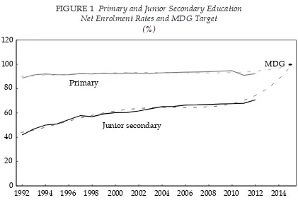
During 1992–2012, net enrolment rates in primary education in Indonesia
increased from 88.7% to 92.4% (igure 1).1 In other words, Indonesia is close to achieving universal primary education. Access to junior secondary education has
also increased signiicantly since the Nine-Year Basic Education Program was
launched, with the net enrolment rate rising from 50.0% to 70.8% during 1994–
1 The net enrolment rate is the ratio of school-age people enrolled in school to the number of school-age people among the population.
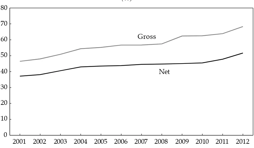
2012 (igure 1). Indonesia’s gross and net enrolment rates in senior secondary
education have also improved, increasing by 21.9 and 14.6 percentage points,
respectively, during 2001–12 (igure 2).2
Higher education in Indonesia has expanded steadily since the 1950s. Between 1975 and 2009, the number of students grew from around 200,000 to more than 4 million. This growth has translated into increased rates of gross enrolment in higher education. During 1975–95, this rate rose from 2% to 9.6%. Then, in the
2000s, it increased from 10.3% to 18.9% (igure 3). Growth in this level of the edu -cation sector has been impressive, though the increases in enrolment rates have been less than those achieved in junior secondary and senior secondary educa-tion.
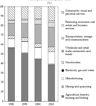
Turning to demand-side considerations, the previous three decades have seen a considerable shift in employment away from the agricultural sector and towards the services, transportation, trade, construction and manufacturing industries. Agriculture’s employment share declined from 56.3% in 1980 to 50.4% in 1990. It then fell further, and by 2010 the agricultural sector’s share of employment had
dropped to 38.4% (igure 4).
2 The gross enrolment rate is a comparative igure for the number of students at a certain stage of education, compared with the number of school-age people among the population, expressed as a percentage. It differs from the net enrolment rate mainly because some stu-dents commence schooling later than the oficial age, and because some stustu-dents repeat classes.
FIGURE 1 Primary and Junior Secondary Education Net Enrolment Rates and MDG Target
(%)
Source: 1992–93 data, Stalker (2007); 1994–2012 data, BPS (2013).
Note: MDG = Millennium Development Goal, which aims to ensure that by 2015 all Indonesian chil-dren will be able to complete primary and junior secondary education.
FIGURE 3 Gross Enrolment Rates in Higher Education, 1975–2012 (%)
Source: 1975–85 data, Lee and Healy (2006); 1995–2012 data, BPS (2013).
FIGURE 2 Gross and Net Enrolment Rates in Senior Secondary Education, 2001–12 (%)
Source: BPS (2013).
During 1980–2010, the following sectors expanded quickly, absorbing a signii -cant number of workers from the declining agricultural sector: transportation, storage and communication; construction; wholesale trade, retail trade, and
res-taurants and hotels; services (inancing, insurance, real-estate and business ser -vices, together with community, social and personal services); and manufacturing. The changing employment structure of the Indonesian economy will affect wage outcomes and the returns to schooling, as particular sectors make more intense use of workers with particular skills. For example, Newhouse and Suryadarma
(2011: 313) note that growth in the industrial sector would inluence the indus -trial and technical majors typically chosen by males in vocational schools. Growth in the services sector would favour majors such as business and tourism, which tend to be chosen by females in vocational schools. The employment structure, FIGURE 4 Share of Population Aged 15 and Over Who Worked during the Previous
Week, by Main Industry, 1980–2010 (%)
$'&'$!$%&$* ' & % #'$$* '&'$
&$&*% )&$ ! %&$'&!
!% $& &$$%&'$ &% !&%
$ %"!$&&! %&!$ !' &! %'$ $ %&& '% %% %$(%
!' &*%! "$%! %$(%
Source: BPS, National Labour Force Survey (Sakernas) (1980, 1990, 2000), and authors’ calculations based on data from BPS (2010).
measured using either occupation or industry of employment, has been used to
capture demand-side inluences on labour-market outcomes for workers at dif -ferent levels of education since the work of Freeman (1977). Below, this article investigates whether the considerable expansion of the education sector, as docu-mented above, along with the shifts in employment across sectors, has affected the returns to schooling in Indonesia.
LITERATURE REVIEW
Studies of the return to schooling in Indonesia have used a number of data sets and employed the methods usually applied in studies of earnings determina-tion in developed countries. Deolalikar (1993) used data from the 1987 Nadetermina-tional Socio-Economic Survey (Susenas) and the 1986 Village Potential Survey (Podes). He used nine dichotomous variables for the different schooling categories in his earnings equation – namely, some primary schooling, completed primary school-ing, general lower secondary schoolschool-ing, vocational lower secondary schoolschool-ing, general higher secondary schooling, vocational higher secondary schooling, diploma 1 or 2, diploma 3, and university.3 The returns to schooling ranged from around 10%, for workers with some primary schooling, to close to 20%, for work-ers with secondary or higher education.4 Generally, however, the results suggest
that adult female workers have signiicantly higher returns to schooling than
adult male workers at the secondary and tertiary levels.
Dulo (2001) studied the impact of the Primary School (Sekolah Dasar, SD) Pres-idential Instruction (Inpres)5 program on the relationship between educational attainment and wages. She used data from the 1995 Intercensal Survey (Supas), though these were restricted to adult males born between 1950 and 1972. She linked the individual-level data on education and wages with district-level data on the number of new primary schools built by SD Inpres between 1973–74 and 1978–79 in the surveyed worker’s region of birth. The framework for this study involved comparing the educational attainment and wages of individuals who had little or no exposure to the Inpres program (that is, those aged between 12 and 17 in 1974) with those of workers who were exposed the entire time they were in primary school (aged between two and six in 1974), in ‘high program’ and ‘low program’ regions. The number of schools built in the worker’s region of birth and the worker’s age when the program was launched were used to deter-mine their exposure to the program. Interactions between dummy variables of an individual’s age in 1974 and the intensity of the program in their region of
3 Deolalikar (1993) used both OLS and selectivity-corrected estimations but noted that the ‘analytical basis for identifying sample selection is weak’ (p. 912), and hence placed more emphasis on the OLS estimates.
4 In order to capture the possibility that the education of workers schooled in earlier time periods may be less relevant to the requirements of the contemporary labour market (termed a cohort effect), Deolalikar’s (1993) estimating equation included an interaction term between the age variable and the education-level dummy. The returns to schooling were typically larger for older cohorts.
5 In 1973, the Indonesian government launched a major primary-school construction pro-gram, SD Inpres. Between 1973–74 and 1978–79, more than 61,000 primary schools were constructed, an average of two schools per 1,000 children aged between ive and 14 in 1971.
birth were used as instruments in the wage equation, and had good explanatory
power. Dulo’s (2001) two-stage least-squares estimates of the economic returns
to education ranged from 6.8% to 10.6%. These estimates were close to, and not
signiicantly different from, those of ordinary least squares (OLS).
Comola and Mello (2010) used data from the 2004 Sakernas in their study of earnings determination, in which they aimed to address selection bias and the endogeneity of educational attainment in the wage equation. They used several approaches to tackling selection bias, including using multinomial and binomial selection equations. They addressed the endogeneity of educational attainment by instrumenting years of schooling in the earnings equation by exposure to Inpres, measured as the intensity of school construction in an individual’s district of birth, and their age when the program was launched, which is similar to the approach
of Dulo (2001). However, they used a single continuous-years-of-education vari -able in their estimating equation. The estimate of the return to education from a Mincerian wage equation for 2004 obtained by standard OLS ranged from 9.5% to 10.3%. Using the binomial selection procedure and Heckman’s (1979) approach, the estimate of the return to education ranged from 10.8% to 11.6%. The return to education obtained by using the multinomial selection procedure ranged from 10.2% to 11.2%. These estimates of the return to education for 2004 are comparable
with the interval of 6.8% to 10.6% reported by Dulo (2011) for 1995. A reason
-ably constant payoff to education is consistent with Van der Eng’s (2010) indings
based on his analysis of Sakernas data from 1989 to 1999.
Newhouse and Suryadarma (2011) compared the earnings returns to vocational and general secondary education in Indonesia, using data from four waves of the Indonesia Family Life Survey (IFLS) (1993, 1997, 2000 and 2007) and distinguish-ing between public and private schools. On the basis of estimations conducted on data pooled across the four waves, they reported a distinct public-school earn-ings premium among males but little evidence of a difference between vocational and general schooling. Among females, however, vocational schooling was rela-tively well rewarded, though the authors provided mixed evidence of the private-versus-public nature of schooling. Examining changes over time by using a model that distinguished cohort effects from age effects brought imprecisely determined estimates, which meant that the most emphasis was placed on general patterns. These indicated that the returns to public vocational education for males have been declining over time, which presumably explains the mixed pattern in the analyses pooled across cohorts.
Patrinos, Ridao-Cano and Sakellariou (2006, 2009) covered the returns to edu-cation in Indonesia in 2003 as part of a study of a number of East Asian and South American countries. Two aspects of their study are directly relevant to this arti-cle: individual heterogeneity in the returns to education,6 and the return at the different levels of education. They use quantile regression to address the former, on the basis that individuals at a particular quantile in the wage distribution will be more homogeneous in unobservables that affect earnings. Accordingly,
6 This is one of two main issues raised by Card (1999). The other – whether the usual estimates of the effects of education are causal – was not addressed, owing to the limited nature of the instruments available, though Patrinos, Ridao-Cano and Sakellariou (2006) argued that ‘while theoretically schooling cannot be taken as exogenous in Mincer equa-tions, empirical results suggest that the extent of the bias may be small’ (p. 4).
examining patterns in the return to education across the wage distribution can determine whether these unobservables interact with education. These studies also reported that Indonesia showed only a modest difference, of around 10%, in the return to education at the top (90th percentile) and bottom (10th percentile) of the wage distribution. In other words, they showed that estimates of the average return to education in Indonesia are not distorted in any major way by unob-served heterogeneity.7
Like Deolalikar (1993), Patrinos, Ridao-Cano and Sakellariou (2006) reported that the return to education in Indonesia at the tertiary level is greater than that at
the primary level. The difference in this return, of around ive percentage points,
was less than that reported in Deolalikar’s (1993) study for 1987, which was based
on a lexible speciication of the earnings equation involving dummy variables.
Whereas Deolalikar suggested that the return to schooling in Indonesia was around 10% at the primary level and close to 20% at the secondary level, Patri-nos, Ridao-Cano and Sakellariou (2006), for 2003, reported lower and fairly stable returns across the wage distribution, suggesting a minor role for the interaction
of unobserved worker heterogeneity and education. However, Dulo (2001) and
Comola and Mello (2010) reported returns to schooling of around 10% for 1995 and 2004, respectively, using a single continuous-years-of-education variable in their estimating equation. These estimates do not appear to be sensitive to selec-tion bias.
Comparing the estimates reported by Deolalikar (1993) and Patrinos, Ridao-Cano and Sakellariou (2006, 2009) suggests that the returns to education in
Indo-nesia have declined between 1987 and 2003, but the similarity of Dulo’s (2001) and Comola and Mello’s (2010) indings suggests that the large-scale expansion of
the Indonesian education sector in recent decades had little effect on the average payoff to the investment in schooling. Newhouse and Suryadarma’s (2011) evi-dence of a decline in earnings rewards for public vocational education for males, and a slight improvement in these rewards for females, was argued by Newhouse and Suryadarma (2011: 299) to be inconsistent with supply-side interpretations.
Below, this article investigates whether this inding holds with the more general
approach adopted by Deolalikar (1993), which enables an assessment of supply-side effects across a wider spectrum of education levels.
CONCEPTUAL FRAMEWORK AND DATA Conceptual framework
The empirical analyses in this article are based on a lexible speciication of the
human-capital earnings equation which incorporates dummy variables for differ-ent education levels – namely, primary school, junior secondary school, vocational senior secondary school, general senior secondary school, college, undergraduate
degree and master’s degree. This more lexible approach offers advantages where
7 Differences between OLS and instrumental variable (IV) estimates obtained using fea-tures of the school system could be due to heterogeneity in the returns to education (Card 1999: 1841). From this perspective, the limited variability in the return to schooling re-ported by Patrinos, Ridao-Cano and Sakellariou (2009) is consistent with the similarity of the OLS and IV estimates reported by Dulo (2001).
the rate of return varies across education levels, and particularly where the aim is to investigate the effect of policy changes that may have had a differential impact
across these levels. This modiied human-capital earnings equation can be written
as follows:
ln(earningsi)=β0+∑kβ1kS.Dumik+β2expri+β3expri 2+β
4tenurei+β5tenurei
2+
β6femalei+β7marriedi+β8urbani+νi
(1)
where earningsi denotes the earnings of individual i,S.Dumikconsists of the dum-mies for education level k, expridenotes years of general labour-market experience,
tenurei represents the job tenure for individual i, femalei is a dummy variable for the gender of individual i, marriedi is a dummy variable for marital status for individual i, and urbani is a residential dummy (urban versus rural) for individual i. Estimates are discussed from a model where the three tertiary qualiications of college, undergraduate degree and master’s degree, each of which has small representation in the sample, are represented by a single variable for the tertiary
qualiied.
The irst variable of labour-market experience, expri, simply records the num-ber of years since the individual left school, as a general measure of potential labour-market experience. The second, tenurei, represents the individual’s years of
experience in their present job and is usually viewed as a measure of irm-speciic
training and knowledge. The gender variable captures gender discrimination, the effects of intermittent labour-force attachment, and the earnings consequences of unobserved trade-offs between work, home duties and leisure that are correlated with gender. The marital-status variable records any consequences of household specialisation for earnings. The specialisation hypothesis argues that married couples often engage in separate household tasks, with male workers focusing on labour-market activities (Gray 1997) while females, having relatively low mar-ket wages, allocate proportionally more time to home duties. Therefore, being married most likely increases the wages of males, while reducing the wages of
females. The inal variable is a residential dummy (rural versus urban), which is
intended to control for the earnings differential between urban and rural areas. The age variable is often a better measure of cumulative labour-market activity than that of potential labour-market experience in situations where the individual has a marginal attachment to the labour market, as is sometimes the case with
women (Blinder 1976). Estimations using the age variable revealed similar ind -ings to those based on potential labour-market experience, as reported below.
Equation (1) uses OLS in its estimations, which may produce biased indings
(owing to the sample of workers not being randomly selected from the popula-tion). Following a two-step Heckman (1979) procedure, however, can address this
potential selection bias: irst, by estimating a probit model of the employment
probability; and, second, by including the derived inverse Mills ratio (λ) as an additional explanatory variable in the earnings function. The inverse Mills ratio is a non-linear function of the explanatory variables included in the employment probability model. As such it is possible to include the same explanatory variables in both the probit model of employment probability and the earnings equation,
and have the inverse Mills ratio term identiied through its inherent non-linearity (termed functional form identiication). However, this is generally viewed as
offering only a weak form of identiication. A stronger form of identiication is
achieved when some variables are included in the employment probability model
that are not in the earnings equation (termed variable identiication). Four vari
-ables were considered in order to have variable identiication, namely household size, a dummy variable for the presence of a child younger than ive in the house -hold, a dummy variable for religion, and a dummy variable for the presence of either a father or a mother in the household.
We used the above approach to sample selection in obtaining our estimates, but in this article we discuss only the OLS results. This is for two main, and related,
reasons: irst, because of the general disquiet in the literature over the robustness
of the sample-selection correction (Puhani 2000; Stolzenberg and Relles 1997); and, second, because of the arguably arbitrary nature of the the variables that are included in the employment probability model but which are not part of the earnings equation in the current set of analyses – even though our testing sug-gested that these restrictions suit our purposes, we have used substantive, rather than technical, grounds in deciding on the exclusion restrictions. The absence of a
correction for sample-selection bias in the intertemporal comparisons is justiiable
if the nature of the sample selection is invariant over time (though this invariance needs to be assumed, because it cannot be shown empirically).
A possible limitation of the analyses is the potential endogeneity of the school-ing variables. Card concluded his 1999 survey of the literature on the causal relationship between education and earnings as follows: ‘Consistent with the summary of the literature from the 1960s and 1970s by Griliches (1977, 1979), the average (or average marginal) return to education in a given population is not much below the estimate that emerges from a simple cross-sectional regression of earnings on education’. Patrinos, Ridao-Cano and Sakellariou (2006, 2009) argued
that the empirical evidence is consistent with a small endogeneity bias. Dulo
(2001) and Comola and de Mello (2010), who used a single continuous-years-of-education variable in their earnings equation, similarly reported that instrumen-tal variable estimates were about the same as the OLS estimates of the return to schooling in Indonesia. Hence, while we cannot, in this article, formally address endogeneity, owing to the limited number of potential instruments where there are multiple schooling variables in the earnings equation (a practical considera-tion that also characterises studies by Deolalikar (1993) and Patrinos, Ridao-Cano and Sakellariou (2006)), the available evidence suggests that the OLS estimates are likely to be very good guides to the true return to schooling.
A further possible limitation of this analysis is that the derivation of an esti-mate of the return to schooling for the average worker may not be useful if the returns around this mean effect vary. Patrinos, Ridao-Cano and Sakellariou (2009) reported, however, that the pay-off to schooling in Indonesia is reasonably stable across the earnings distribution, suggesting that a focus on only the mean effect of
years of education should not limit this analysis signiicantly.
The potential for province-speciic factors to affect the estimates of the return
to schooling also needs to be accommodated. The standard way of addressing this concern is to include dummy variables for the province of residence in the estimating equation, though it appears that most of the empirical research for Indonesia does not address this issue (possibly because of endogeneity concerns associated with the choice of location of residence). Using dummy variables for
the province of residence to re-estimate the models below has little impact on the estimates of the returns to education, other than at the university level, and does not affect the pattern of changes over time. Estimates from models that omit the dummies for province of residence are also presented below.8
To calculate the rate of return to an additional year of schooling under this lex -ible approach, one of two methods may be used. First, one may follow Deolalikar (1993):
r
k =
βk
n
k
(2)
where βk is the coeficient of a speciic level of education and nk is the number of years required to complete this level.9 This is an average return.
Second, one may follow Sakellariou (2003), El-Hamidi (2005), and Kimenyi,
Mwabu and Manda (2006), by dividing the difference between the coeficients
of adjacent schooling levels by the difference in the years of schooling associated
with these levels. Hence, in this speciication, the private rate of return to educa -tion at the kth level of education is as follows:
r
k =
βk−βk−1
(
)
Δn k
(3)
where ∆nk is the difference in the years of schooling between education levels k and k–1. This approach focuses on a marginal return. As equation (2) can be sensi-tive to the earnings position of the excluded education group, we report below
only the indings from equation (3) (although both approaches yield a consistent
story).
Data source
This article uses two waves of IFLS in its empirical analysis: IFLS1 (ielded in 1993) and IFLS4 (ielded in 2007–08). IFLS is a nationally representative sample
comprising 7,224 (IFLS1) and 13,536 (IFLS4) households, spread across prov-inces on the islands of Java, Sumatra, Bali, West Nusa Tenggara, Kalimantan and Sulawesi. Together, these provinces encompass approximately 83% of the Indonesian population and much of its heterogeneity. IFLS1 was administered
by the RAND Corporation, in collaboration with Lembaga Demograi Univer -sitas Indonesia, Jakarta. IFLS4 was a collaborative effort by RAND, the Center for Population and Policy Studies at the University of Gadjah Mada, and Survey Meter. For our analyses of the returns to schooling in Indonesia, we restricted our
8 A parallel set of estimates of the returns to levels of education, based on the models aug-mented with dummy variables for the province of residence, is available from the authors on request.
9 The number of years of study required to complete primary school in Indonesia is six, followed by three years of junior secondary school, three to four years of either vocational senior secondary school or general senior secondary school, and three years of college. An average of four years is needed for a bachelor’s (undergraduate) degree, and an additional two years for a master’s degree.
TABLE 1 Deinition of Variables
Ln (earnings) Logarithm of monthly earnings
education level Dummy variables, with a reference group of those who did not inish primary school
expr Potential labour-market experience
expr2 Square of potential labour-market experience
tenure Experience in present job
tenure2 Square of experience in present job
female Dummy variable: 1 = individual is female; 0 = other married Dummy variable: 1 = individual is married; 0 = other
urban Dummy variable: 1 = individual lives in urban area; 0 = other
sample to workers aged 15–65 who were not full-time students, who reported non-missing labour income and who provided information on their schooling. We omitted those persons serving in the military during the survey week, because
the wages of those in the armed services do not necessarily relect market forces.
Our analysis includes the 5,508 observations from 1993 and 4,596 observations from 2007–08 that satisfy these criteria. The construction of the main variables is
discussed below, and the deinitions are given in table 1.
The dependent variable in our analysis is the natural logarithm of monthly
earnings, or the value of all beneits secured by a worker in their job. We have
used monthly earnings instead of an hourly earnings indicator because survey respondents were explicitly asked to supply the former.10 Employer–employee agreements in Indonesia are also generally based on monthly wages. The use of an hourly-wage dependent variable is shown in a set of supplementary estima-tions (not reported here) to be associated with a modest reduction (of around one percentage point) in the estimated return to schooling, which is reasonably uniform across the levels of education and time periods that we consider in our analysis.
There are three main differences that hinder comparisons between the IFLS1
data and the IFLS4 data: irst, a job-tenure variable cannot be constructed for the
IFLS1 data; second, the coding of education levels differs, so although an under-graduate degree and a master’s degree may be considered separately in the IFLS4 data, they need to be combined when examining the IFLS1 data; and, third, a more precise measure of potential labour-market experience can be constructed with the IFLS4 data than with the IFLS1 data. In particular, the measure of potential labour-market experience for the IFLS1 data relies on the formula of age, minus
years of schooling, minus oficial age of starting primary school (six or seven),
whereas the IFLS4 data can provide the more accurate measure of age, minus
years of schooling, minus age irst attended primary school.
The difference in the coding of education variables is of reasonably minor importance (given the small number of surveyed individuals with master’s degrees), as is the difference in the algorithms for the construction of the variable
10 The calculation of hourly wages from monthly earnings would require using another variable, the number of hours worked in the reference month, which would be subject to measurement error.
of potential labour-market experience. The omission of the tenure variable is
important, however, because it is a highly signiicant determinant of earnings in
the IFLS4 data. Hence, we analysed the IFLS4 data using an estimating equation that includes the variables of both tenure and the master’s degree level, as well as the more precise variable of potential labour-market experience. To compare the data over time, we re-estimated the equations for the IFLS4 data by using a
restricted speciication that matched the data, where possible, with those of IFLS1. This approach also enabled us to test the sensitivity of the results to this speciica -tion.
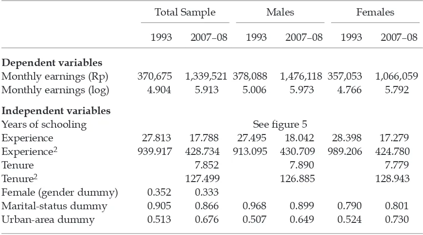
Table 2 reports the summary statistics for the main variables. The mean total monthly earnings of the surveyed workers are Rp 370,676 (IFLS1) and Rp 1,339,521 (IFLS4). The workers in the sample have mean labour-market experi-ence of approximately 27.81 years (IFLS1) and 17.79 years (IFLS4).11 The mean length of job tenure is 7.85 years. The data in table 2 reveal that male and female workers have broadly similar levels of potential labour-market experience and job tenure. They differ appreciably in terms of earnings, however, where the mean for males (Rp 1,476,118) is 38.5% higher than the mean for females (Rp 1,066,059).
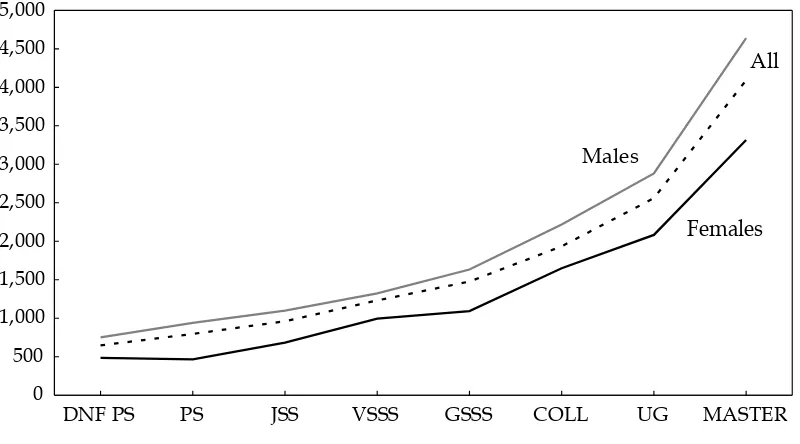
Figure 5 describes the composition of the IFLS4 sample on the basis of
educa-tion level and igure 6 provides a preliminary examinaeduca-tion of the importance of education level to earnings determination. The patterns in igure 6 coincide with
the main prediction of human-capital theory, which states that more educated workers earn more as a result of improved productivity. Female workers have lower average monthly earnings than their male counterparts at all education levels, but, in percentage terms, the gender gap in earnings generally tends to
11 The difference in years of potential labour-market experience is due to the higher mean age in IFLS1 and the difference in the way that this variable is calculated in each wave, as described in the text.
TABLE 2 Summary Statistics of Main Variables
Total Sample Males Females
1993 2007–08 1993 2007–08 1993 2007–08
Dependent variables
Monthly earnings (Rp) 370,675 1,339,521 378,088 1,476,118 357,053 1,066,059 Monthly earnings (log) 4.904 5.913 5.006 5.973 4.766 5.792
Independent variables
Years of schooling See igure 5
Experience 27.813 17.788 27.495 18.042 28.398 17.279 Experience2 939.917 428.734 913.095 430.709 989.206 424.780
Tenure 7.852 7.890 7.779
Tenure2 127.499 126.885 128.943
Female (gender dummy) 0.352 0.333
Marital-status dummy 0.905 0.866 0.968 0.899 0.790 0.801 Urban-area dummy 0.513 0.676 0.507 0.649 0.524 0.730
Source: Authors’ calculations based on IFLS1 and IFLS4 data.
FIGURE 5 Distribution of Education Level, IFLS4 (2007–08) (%)
! !
Source: Authors’ calculation based on IFLS4 data.
Note: DNF PS, did not inish primary school; PS, primary school; JSS, junior secondary school; VSSS,
vocational senior secondary school; GSSS, general senior secondary school; COLL, college; UG, under-graduate degree; MASTER, master’s degree.
FIGURE 6 Mean Monthly Earnings by Education Level and Gender, IFLS4 (2007–08) (Rp ‘000)
Source: Authors’ calculations based on IFLS4 data.
Note: DNF PS, did not inish primary school; PS, primary school; JSS, junior secondary school; VSSS,
vocational senior secondary school; GSSS, general senior secondary school; COLL, college; UG, under-graduate degree; MASTER, master’s degree.
decrease as the level of education rises: primary school (51%), junior secondary school (38%), vocational senior secondary school (25%), general senior secondary school (33%), college (26%), undergraduate (28%) and master’s degree (28%).
EMPIRICAL RESULTS
OLS estimates based on IFLS4 (2007–08)
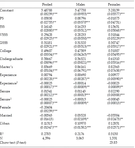
Table 3 presents the OLS estimates of the earnings equation. As noted above, the
speciication of the estimating equation used for the IFLS4 data contains several
variables that are not available for the IFLS1 data. We have presented estimates based on ILFS4 from models that include the variables which are not available in IFLS1 to facilitate discussion of a broader range of earnings effects.
The estimated coeficients are jointly signiicant in each estimation, as indi -cated by the F-test. The R2 values, of between 0.21 and 0.32, are typical for cross-sectional earnings equations of this type. Most of the partial effects are estimated with statistical precision, and have the expected signs.
Table 3 suggests that tenure has a greater impact than potential labour-market
experience on earnings for all speciications (pooled, males and females). Among
labour-market entrants (experience and tenure = 0), the increase in earnings asso-ciated with potential experience is 0.79%, 0.69% and 0.98% for the pooled, male and female samples, respectively. The return to job tenure, however, is 1.54%, 1.14% and 2.29% for these samples. For those workers with 10 years of potential labour-market experience and job tenure, the increase in earnings associated with additional potential experience is 0.29%, 0.41% and 0.52% for the pooled, male and female samples, respectively, and the increase in earnings associated with additional job tenure is 1.04%, 0.84% and 1.39%.
The marital-status variable is signiicant only when the male and female sam
-ples are examined separately, and it is not signiicant for the speciication esti -mated using the combined sample of males and females (presumably because of the pooling of two samples that are characterised by opposing effects of the married variable). Being married has a positive effect on earnings for males and a negative effect on earnings for females, which may be evidence in support of the specialisation hypothesis. By being married, male workers can devote more of their time and effort to labour-market activities and, as a result, increase their earnings. In contrast, being married decreases the earnings of female workers, presumably because they then spend more time on home duties, as well as having and raising children.
The estimates for the dummy variable for the urban area of residence suggest
that, on average, residents of urban areas earn signiicantly more than those of the rural areas. The coeficient of the urban-dummy variable is 0.10970 for males and
0.12851 for females, which shows that male workers from urban areas earn around 11% more than those from rural areas, and that female workers from urban areas earn around 13% more than those from rural areas.
The education level chosen as the benchmark, and hence omitted from the
esti-mating equation, is the lowest education level, ‘Did not inish primary school’.
The other education levels in our model form a hierarchy, from lowest to
high-est. Hence, we expect that the estimated coeficients will all be positive, and will
increase in magnitude as one reads down the table. All but one of the education
variables is associated with statistically signiicant partial effects, the exception being the coeficient for females who completed primary school.12 The F-test
conirms that the coeficients of education-level variables for males and females
12 Replacing the variables for potential labour-market experience with the age variables sees most of the coeficients of the education-level dummy variables decrease for all sam-ples. Blinder (1976) reports a similar inding.
TABLE 3 OLS Estimates of Earnings Functions with Level-of-Education Dummy Variables, IFLS4 (2007–08)
Source: Authors’ calculations based on IFLS4 data.
Note: OLS = ordinary least squares. Standard errors are in parentheses. The Chow test gauges whether the structure of the wage-determination process for females differs from that for males. PS, primary school; JSS, junior secondary school; VSSS, vocational senior secondary school; GSSS, general senior secondary school.
* p < 0.1; ** p < 0.05; *** p < 0.01
are statistically different. The fact that the value of the constant term is higher for males than for females indicates that males, without schooling and labour-market experience, earn more than comparable females, and suggests that wage discrimi-nation is taking place against females in the labour market. It is consistent with the estimate of the gender effect in the pooled sample.
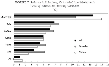
Based on the results in table 3, the return to schooling for each education level can be calculated using equation (3). Figure 7 presents the marginal return to com-pleting each additional level of education – for example, junior secondary school compared with primary school, and general senior secondary school compared with junior secondary school. These results show that the return in private earn-ings to additional years of schooling in Indonesia increases with the level of edu-cation.
All of these returns are substantially lower than the average returns to school-ing in Asian countries. Psacharopoulos (1981, 1985, 1994) found that the returns to schooling for Asian countries are 31%–39% for primary education, 15%–19% for secondary education and 18%–20% for tertiary education. Moreover, these esti-mates of the return to schooling in Indonesia are much lower than those reported by Deolalikar (1993) for the late 1980s, and lower than those presented by Patri-nos, Ridao-Cano and Sakellariou (2006) for 2003.
The gender differences presented in igure 7 could be due to a number of labour-market inluences. Ren and Miller (2012), for example, investigated the
gender differential in the average return to schooling in China, and argued that it could be due to worker self-selection, a more limited supply of skilled female workers, differential technological requirements in fedominated and male-dominated jobs, and discrimination against female workers that is less intense among the better educated. The higher return for males than for females at both
FIGURE 7 Returns to Schooling, Calculated from Model with Level-of-Education Dummy Variables
(%)
Source: Authors’ calculations based on data shown in table 3.
Note: PS, primary school; JSS, junior secondary school; VSSS, vocational senior secondary school; GSSS, general senior secondary school; COLL, college; UG, undergraduate degree; MASTER, master’s
degree. The primary-school coeficient for the female sample is statistically insigniicant.
the master’s degree and primary-school levels in Indonesia suggests that limited importance should be attributed to self-selection and discrimination. Addition-ally, self-selection appears to have only a minor role in earnings determination in Indonesia. Ren and Miller (2012) investigated the potential impact of other
possi-ble inluences on the return to education, using a decomposition of the difference
in the average pay-off to schooling for two groups developed by Chiswick and Miller (2008). Chiswick and Miller’s (2008) research, however, was based on a sin-gle continuous-years-of-education variable, and their framework does not extend
to the lexible speciication of the earnings equation involving multiple dummy
variables for level of education used in the current set of analyses.13
We considered several extensions to this set of analyses, including, in the irst
instance, using Heckman’s two-step approach to selection correction. In these estimates, the selectivity term (λ) was signiicant only at the 10% level, and the
signs and signiicance of the schooling coeficients were broadly similar across
both the uncorrected earnings functions (table 3) and the selection-corrected earn-ings functions. In other words, it seems that sample selection bias is not a serious problem in this article, though the limitations of this approach need to be kept in mind.
The second extension involved replacing the variables for those workers who have completed college, those with an undergraduate degree and those with a master’s degree (which all have small representations in the sample) with a single
variable for the tertiary qualiied. This modiication made no changes of any con -sequence to the return to schooling at the primary, junior secondary, vocational senior secondary and general senior secondary levels. The return to schooling for
the tertiary qualiied in the pooled, male and female samples is 6.8%, 6.3%, and
7.3%, respectively.
Comparisons between IFLS1 (1993) and IFLS4 (2007–08)
Comparing our results with those of Deolalikar (1993) and Patrinos, Ridao-Cano and Sakellariou (2006) suggests that the returns to schooling in 1987 and 2003 are both greater than those in 2007–08. The two previous studies, however, rely on a different data source (Susenas) from those used in this article, and used different sets of explanatory variables in their estimating equations, so these comparisons
could relect these differences rather than the changes over time in the proitabil -ity of the investment in education. To gain more solid evidence on whether the returns to schooling in Indonesia have changed over time, we compare estimates
based on data from the irst and fourth series of the IFLS. As discussed above, a
lack of comparable data forced us to make several changes to the estimating equa-tion, including deriving potential labour-market experience by using the conven-tional formula of age, minus the number of years of schooling, minus 7 (for both sets of data); excluding the tenure variables from the model; and, as IFLS1 does not include master’s degrees in its education categories, combining
undergradu-ate and master’s qualiications into one education level (university).
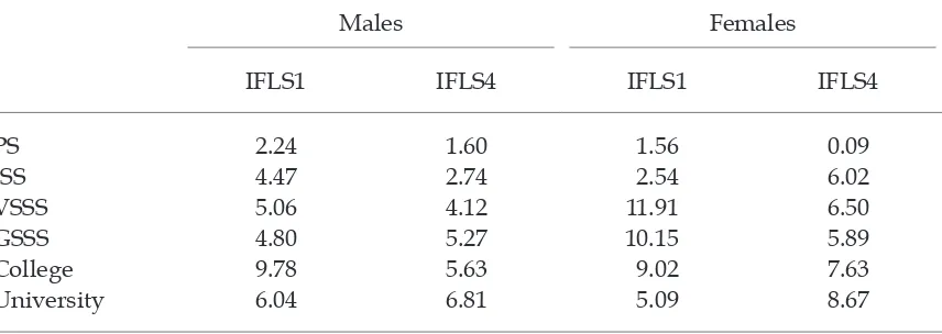
Table 4 compares the estimated returns to schooling based on IFLS4 data, using
this modiied model of earnings determination and estimated returns to schooling
13 Applying the approach of Chiswick and Miller (2008) to the average return to schooling for various groups in the Indonesian labour market is a topic for future research.
obtained from an identical model applied to IFLS1 data. The return to education has fallen in eight of the 12 categories, but several of the changes across time peri-ods are quite minor – for example, the return to primary schooling for males. A number of the changes, however, are more substantial, such as the reduced return for both males and females to college education and the increased return to a uni-versity degree. In two of the four categories in which the return to education has risen – junior secondary school, for females, and general senior secondary school, for males – the return for the other gender fell.
These results, in general, support our inding that the returns to schooling for
Indonesia have declined in recent years. However, the gaps between the returns to schooling based on IFLS1 data and those based on IFLS4 data are not as wide as those revealed by the comparisons with the two earlier studies mentioned above, and this conclusion does not apply to university degrees. In addition, the changes
over time are not as regular when conined to a discussion of differences between
results obtained from comparable data sets.
Cohort versus age effects
Newhouse and Suryadarma (2011) argued that changes in the pay-off to
educa-tion over time can relect both cohort and age effects. A cohort effect arises when
workers in a particular age bracket (for example, those aged 30–34) and born in a
certain period (for example, during the 1960s) have a different return to a speciic
level of education than workers born earlier (for example, during the 1950s). Age effects can be documented by following a particular cohort over time and identi-fying any changes in returns. This type of analysis needs data collected at two or more points in time, and implementing it requires cohorts with broad member-ships in each data set. We follow Newhouse and Suryadarma (2011) in consider-ing three cohorts: oldest (born in 1940–62), middle (born in 1963 –72) and youngest
(born in 1973–80). The IFLS1 and IFLS4 data are irst pooled (with earnings in
1993 indexed to 2007 values, using the BPS urban price index) and then parti-tioned according to these three cohorts. The earnings equation is then estimated
TABLE 4 Returns to Education between IFLS1 (1993) and IFLS4 (2007–08) (%)
Males Females
IFLS1 IFLS4 IFLS1 IFLS4
PS 2.24 1.60 1.56 0.09
JSS 4.47 2.74 2.54 6.02
VSSS 5.06 4.12 11.91 6.50
GSSS 4.80 5.27 10.15 5.89
College 9.78 5.63 9.02 7.63
University 6.04 6.81 5.09 8.67
Source: Authors’ calculations based on IFLS1 and IFLS4 data.
Note: PS, primary school; JSS, junior secondary school; VSSS, vocational senior secondary school; GSSS, general senior secondary school.
within each cohort, with separate education terms for each survey period.14 Many of Newhouse and Suryadarma’s (2011) estimates were imprecisely determined
(only 13%–50% were statistically signiicant), and hence they placed more empha -sis on broad patterns. We take a similar approach here.
Estimates of the cohort model have two general features: irst, nearly all (97%) of the estimated changes over time in the education coeficients within each cohort are negative; second, relatively few (28%) of these estimated coeficients are sta
-tistically signiicant. There are a greater number of signiicant education × survey interaction terms for the older cohort than for the younger cohort, and for the pooled sample analyses than for the estimates undertaken separately for males and females. The negative education × survey effects indicate that earnings decline as older age groups within a given cohort are considered, which is consistent with obsolescence of human-capital skills.
Given the imprecise nature of the estimated coeficients (especially in analyses
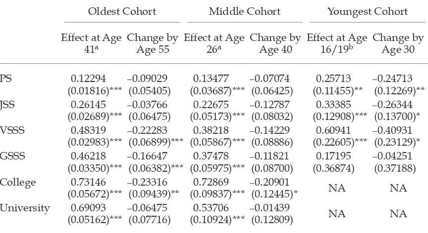
by gender) that are of primary interest to this article, we present only general comments on the estimates from the combined sample of males and females.15 Table 5 presents selected estimates from this approach. There are three parts to
this table, one each for the older, middle and younger cohorts deined above. For each cohort there are two columns of results. The irst column is the effect of the
particular level of education on earnings that was recorded in IFLS1 (1993), and the second is the change in this effect between IFLS1 and IFLS4 (2007–08).
Table 5 shows that the earnings advantage in IFLS1 of those in the oldest cohort who completed primary school was 12.3%, compared with the benchmark group (those who did not complete primary school). These individuals were, on aver-age, 41 years old during IFLS1. In IFLS4, when the individuals were around 55 years old, this earnings advantage had all but disappeared (having declined by 9.03 percentage points). The middle cohort displays a similar pattern – their earn-ings advantage in IFLS1 was 13.5% but had declined by 7.07 percentage points by IFLS4. The earnings advantage of the youngest cohort in IFLS1, at 25.7%, was much higher than that of the other cohorts (owing to less time having elapsed since the youngest cohort left school). By IFLS4, however, their advantage had dissipated: the most unskilled groups in the labour force (which, according to
igure 5, compose 7% of the sample), who by deinition have few human-capital
skills that could lose value over time, had caught up with their educated coun-terparts.
Turning to the overall patterns in table 5, the earnings effects for the oldest and middle cohorts in IFLS1 are generally higher for the former than they are for the latter (though those having completed primary school are exceptions). Changes in the earnings effects for the middle and youngest cohorts in IFLS1 suggests that relative earnings have increased for those with primary schooling, junior sec-ondary schooling and vocational senior secsec-ondary schooling, and decreased for those with general senior secondary schooling, although the last two rely on only a small number of observations. If we examine the marginal returns, however,
14 Given the ages at which the higher levels of education are typically completed, several education levels are not represented for the youngest cohort in IFLS1 (see also Newhouse and Suryadarma 2011: 310).
15 The full set of results is available from the authors on request.
which rely on differences in the estimated coeficients at the various levels of
education, only primary schooling and vocational senior secondary schooling are associated with improved earnings positions in the younger cohort, compared with the middle cohort. In each instance of decline among the oldest and middle cohorts, its effect on the marginal rate of return is modest.
Examining changes in the education coeficients with age reveals three fea -tures. First, there is little change with age among university graduates, which suggests either that their skills do not deteriorate with age or that they receive ongoing on-the-job training (that is, that university education and further train-ing are complementary). Second, changes for a given cohort, especially for the middle cohort, tend to be uniform across education levels. Consequently, they have only a minimal effect on the marginal return, which is based on the
differ-ences in the education coeficients for the adjacent education levels. There are
exceptions to this general pattern, such as among college-educated individuals, though these can be found in each cohort. Third, the decline with age among those with vocational senior secondary schooling exceeds that among those with general senior secondary schooling in each cohort, which suggests that special-ised skills may lose value more rapidly in a dynamic labour market.
TABLE 5 Estimates of Effects of Level of Education on Earnings from the Cohort
Model, IFLS1 (1993) and IFLS4 (2007–08)
Oldest Cohort Middle Cohort Youngest Cohort
Effect at Age
Source: Authors’ calculations based on IFLS1 and IFLS4 data.
Note: PS, primary school; JSS, junior secondary school; VSSS, vocational senior secondary school; GSSS, general senior secondary school. Standard errors in parentheses. NA = not applicable, owing to the age of the cohort in 1993 (IFLS1).
aMidpoint of age of cohort
bMidpoint of age of the youngest cohort (in PS & JSS/VSSS & GSSS), whose oldest members were 20 in 1993 (IFLS1).
* p < 0.1; ** p < 0.05; *** p < 0.01
In summary, these estimates suggest that cohort and age effects have a modest impact on the returns to education in Indonesia. The cohort effect could stem from unobservable characteristics of the workers, or from changes in the quality of education following the rapid increase in enrolments over the past few decades, whereas the age effect is presumably linked to the obsolescence of human-capital skills. Their presence in all education levels, other than the university level, can be taken to indicate a need for ongoing learning programs that upgrade workers’ skills to meet the evolving demands of the labour market.
CONCLUSIONS
In this article, we have reported evidence on the returns to schooling in Indonesia, and have obtained separate estimates for males and females. We have used OLS as our primary methodological approach, though we also used Heckman’s two-step estimator to correct for the possibility of selection bias. The results suggest
that sample-selection bias was not signiicant in our study.
Our results show that the returns to schooling tend to increase as the level of education increases, which opposes much of the existing empirical evidence (Psacharopoulos 1981, 1985, 1994). They also show that males and females have different patterns of returns at the senior secondary level of education. Males, for example, have a higher return to schooling if they graduated from general senior secondary school rather than from vocational senior secondary school, whereas
females have the opposite pattern. These results complement the indings of other
studies, such as those of Deolalikar (1993).
We found that the returns to schooling in Indonesia are low compared with those in many other countries, particularly in Asian and developing countries.
Our most important inding, however, is that the returns to schooling documented
in this article – that is, those based on IFLS4 data – are generally lower than those computed using earlier data. When compared with Deolalikar’s (1993) estimates
for 1987, for example, our indings for 2007–08 are much lower. Our estimates
are also lower than those of Patrinos, Ridao-Cano and Sakellariou (2006). When compared with a parallel analysis of data from IFLS1, education appears to be a
less proitable investment in 2007–08 than in 1993, though typically by a smaller
magnitude than that suggested by the comparisons with earlier studies. This
con-clusion, however, does not apply to a university degree: the proitability of this
education level increased between 1993 and 2007–08, for both males and females. In addition, there are two other instances (one for males, the other for females) where the return to education rose. In both, these rises were been accompanied by a fall in the return to education for the other gender. Similarly, Newhouse and Suryadarma (2011) found that the return to public vocational education over time in Indonesia has decreased for males but possibly increased for females.
Newhouse and Suryadarma (2011) also suggested that the changes they
docu-mented in the proitability of vocational education could be due to a deteriora
-tion in the quality of voca-tional training in the ields entered by men, as well
as the changes in the Indonesian economy. Between 1980 and 2010, Indonesia experienced a sharp decline in the relative importance of its agricultural sector and increases in the relative importance of the following sectors:
manufactur-ing; services (inancing, insurance, real-estate and business services, together
with community, social and personal services); wholesale trade, retail trade, and restaurants and hotels; construction; and transportation, storage and
communica-tion (igure 4).
A similar explanation could account for the changes documented in this arti-cle. The increasing relative importance of the wholesale trade, retail trade, and restaurants and hotels sector would have favoured labour-market outcomes for females, and a more competitive construction industry would have favoured such outcomes for males. The marginal returns considered in table 4 depend, how-ever, on relative outcomes at adjacent levels of education. For example, growth in employment for males in construction could be associated with either a higher or a lower marginal return to general senior secondary school: it would most likely lower this return if the effect of the growth in employment was more pronounced at junior secondary school than it was at senior secondary school, and it would most likely raise the return if the growth in employment was more pronounced at the level of senior secondary school.
Thus, the role of gender-speciic changes in employment levels across indus -trial sectors would vary by the level of education, depending on the education input–output mix in the industrial sectors. Without detailed input–output tables,
we cannot be more deinitive in this regard. Given general perceptions of the
education mix in the various industrial sectors, however, the relative decline of employment in Indonesia’s agricultural sector, for example, would be expected to have disadvantaged the less well educated, whereas the relative growth of employment in the various services sectors should have favoured the better
edu-cated (which implies an increase in the proitability of an investment in educa -tion).
The general pattern of decline in the proitability of an investment in educa -tion, then, may be attributable to the large-scale expansion of the education sec-tor in Indonesia, or to a rate of expansion in the number of jobs requiring higher educational attainment which lagged behind the expansion of education and the increase of average educational attainment – a similar situation to that dis-cussed in Freeman’s (1977) study for the US. Further demand-side adjustments,
as occurred in the US during the 1980s and 1990s, could enhance the proitability
of the investment in education and so increase the returns to their former levels. Achieving such adjustments should be a priority of current policy.
REFERENCES
Blinder, A.S. (1976) ‘On dogmatism in human capital theory’, The Journal of Human Resources 11 (1): 8–22.
BPS (Central Statistics Agency) (2010) Perkembangan Beberapa Indikator Utama Sosial-Ekonomi Indonesia (Trends of the Selected Socio-Economic Indicators of Indonesia), BPS, Jakarta. BPS (Central Statistics Agency) (2013) Education Indicators, 1994–2012, BPS, Jakarta,
availa-ble at <http://www.bps.go.id/eng/tab_sub/view.php?kat=1&tabel=1&daftar=1&id_ subyek=28¬ab=1>.
Card, D. (1999) ‘The causal effect of education on earnings’, in Handbook of Labor Economics, Vol. 3, eds O. Ashenfelter and D. Card, Elsevier Science, Amsterdam, 1801–63.
Chiswick, B.R. and Miller, P.W. (2008) ‘Why is the payoff to schooling smaller for immi-grants?’, Labour Economics 15 (6): 1317–40.
Comola, M., and de Mello, L. (2010) ‘Educational attainment and selection into the labour market: the determinants of employment and earnings in Indonesia’, Paris-Jourdan Sci-ences Economiques Working Paper 2010-06, Paris-Jourdan SciSci-ences Economiques, Paris. Deolalikar, A.B. (1993) ‘Gender differences in the returns to schooling and in school
enroll-ment rates in Indonesia’, The Journal of Human Resources 28 (4): 899–932.
Dulo, E. (2001) ‘Schooling and labor market consequences of school construction in Indo-nesia: evidence from an unusual policy experiment’, The American Economic Review 91 (4): 795–813.
El-Hamidi, F. (2005) ‘General or vocational? Evidence on school choice, returns, and “sheep skin” effects from Egypt 1998’, Paper presented at the Twenty-Fifth Annual Meeting of The Middle East Economic Association, Allied Social Sciences Association, Philadel-phia, Pennsylvania, 7–9 January.
Freeman, R.B. (1977) ‘The decline in the economic rewards to college education’, The Review of Economics and Statistics 59 (1): 18–29.
Griliches, Z. (1977) ‘Estimating the returns to schooling: some econometric problems’, Econometrica 45: 1–22.
Griliches, Z. (1979) ‘Sibling models and data in economics: beginnings of a survey’, Journal of Political Economy 87: S37–S65.
Gray, J.S. (1997) ‘The fall in men’s return to marriage: declining productivity effect or changing selection?’, The Journal of Human Resources 32 (3): 481–504.
Heckman, J.J. (1979) ‘Sample selection bias as a speciication error’, Econometrica 47 (1): 153–61.
Kimenyi, M.S., Mwabu, G. and Manda, D.K. (2006) ‘Human capital externalities and pri-vate returns to education in Kenya’, Eastern Economic Journal 32 (3): 493–513.
Lee, M.N.N., and Healy, S. (2006) ‘Higher education in South-East Asia: an overview’, in Higher Education in South-East Asia, Asia-Paciic Programme of Educational Innovation for Development, UNESCO, Bangkok, 1–12.
Newhouse, D. and Suryadarma, D. (2011) ‘The value of vocational education: high school type and labor market outcomes in Indonesia’, The World Bank Economic Review 25 (2): 296–322.
Patrinos, H.A., Ridao-Cano, C. and Sakellariou, C. (2006) ‘Estimating the returns to edu-cation: accounting for heterogeneity in ability’, World Bank Policy Research Working Paper 4040, World Bank, Washington DC.
Patrinos, H.A., Ridao-Cano, C. and Sakellariou, C. (2009) ‘A note on schooling and wage inequality in the public and private sector’, Empirical Economics 37: 383–92.
Psacharopoulos, G. (1981) ‘Returns to education: an updated international comparison’, Comparative Education 17 (3): 321–41.
Psacharopoulos, G. (1985) ‘Returns to education: a further international update and impli-cations’, The Journal of Human Resources 20 (4): 583–604.
Psacharopoulos, G. (1994) ‘Returns to investment in education: a global update’, World Development 22 (9): 1325–43.
Puhani, P.A. (2000) ‘The Heckman correction for sample selection and its critique’, Journal of Economic Surveys 14 (1): 53–68.
Ren, W. and Miller, P.W. (2012) ‘Gender differences in the return to schooling in rural China’, Journal of Development Studies 48 (1): 133–50.
Sakellariou, C. (2003) ‘Rates of return to investments in formal and technical/vocational education in Singapore’, Education Economics 11 (1): 73–87.
Stalker, P. (2007) Let’s Speak Out for MDGs Achieving the Millennium Development Goals in Indonesia, National Development Planning Agency and United Nations, Jakarta.
Stolzenberg, R.M. and Relles, D.A. (1997) ‘Tools for intuition about sample selection bias and its correction’, American Sociological Review 62: 494–507.
Van der Eng, P. (2010) ‘The sources of long-term economic growth in Indonesia, 1880–2008’, Explorations in Economic History 47 (3): 294–309.