Estimating Goldfelds Conventional Money Demand Function Using Ridge Regression.

(1)

Estimating Goldfeld’s Conventional Money Demand Function Using Ridge Regression

Maman Setiawan

Abstract

(2)

I. Introduction

Problem of multicollinearity arising from the nature of economic models and data often result in highly unstable and unrealistic estimates of structural parameters, especially if one is restricted to unbiased estimators such as OLS. If this problem is resolved by deleting important variables from the models, one risks a serious omitted-variables-specification bias (Brown and Beattie, 1975). Ridge regression has been known and developed as an alternative prediction method to ordinary least squares regression (OLS) in cases where there is a high degree of multicollinearity among the predictor variables. If the mean square error (MSE) criterion is used as a measure of accuracy, there always exists a more accurate “ridge regression” estimate than the unbiased OLS estimate, as shown by Hoerl and Kennard (1970a, pp.61-63). Estimating Goldfeld’s conventional money demand function is an area where there is a high degree of overlap among the predictor variables and should thus be an excellent area to apply ridge regression instead of the usual OLS regression used (Tracey and Sedlacek, 1983). It has long been recognized that multicollinearity does not hinder and sometimes aids in forecasting as long as the multicollinearity remains in the forecast period. However, in a demand for money equation with several interest rate, a changing term structure may alter the multicollinearity pattern. In such circumstances, ridge estimates which are less affected by multicollinearity may provide better forecasts than OLS estimates (Watson and White, 1976). Obtaining valid prediction equations in this area is often difficult because the high degree of multicollinearity tends to create very different prediction equations from year to year. Thus the process of validating these equations typically involves collecting very large samples over many years. Ridge regression has been found to be most effective in exactly these cases. Ridge regression should result in more stable equations with high multicollinear data, and thus, should be more valid using smaller samples than typically required by least squares method.

The purpose of this study was to examine the efficacy of ridge regression over ordinary least squares regression in Goldfeld’s conventional money demand function. This study has two aims : 1). To propose a test of the ability of the ridge regression to forecast. 2) To show that the coefficients of the ridge regression statistically are not different as the OLS coefficients.

II. Literature Review

Some research about the use of Ridge regression had been conducted over the years. According to Darlington (1978) and Faden (1978), Ridge regression was developed to be used in exactly these situations of high multi collinearity. Overall, the OLS and Ridge Regression procedures are identical except that in ridge regression, a small constant is added to the main diagonal of the variance-covariance matrix prior to the determination of the regression equation. This adding of the constant creates a "ridge" on the main diagonal, hence the name. Adding this ridge is an artificial means of decreasing the relative amount of collinearity in the data. The determination of the specific constant (=delta) that is added to the matrix is determined by using an iterative approach; selecting the delta value that results in the lowest total mean square error for the prediction equation.

Consider the normal linear regression model :

Y = Xβ + ε ……….(1)

(3)

unknown and to be estimated by the data, y and X. It is well known that the ordinary least squares (OLS) estimator for is given by :

b = (X’X)-1 X’y ……….(2)

Under the model assumptions, the OLS estimator is the best linear unbiased estimator by the Gauss-Markov Theorem. However, comparing it with non linear or biased estimators, the OLS estimator may perform worse in particular situations. One of these is the case of near multicollinearity, where the matrix X’X is nearly singular. In that situation, the variance of b, given by 2(X’X)-1 , can be very large. A biased estimator with less dispersion may in that case be more efficient in terms of the mean squared error criterion. This is the basic idea of ridge and shrinkage estimators, which were introduced by Hoerl and Kennard (1970) for the above regression model.

Grob (2003) gives an excellent surveys of alternatives to least squares estimation such as ridge estimators and shrinkage estimators. He gives a possible justification that the addition of matrix kIp (where k is scalar) to X’X yields a more stable matrix X’X to kIp and that the ridge estimator of ,

β = (X’X + kIp)-1 X’y ………..(3)

Var-Cov(β) = 2 (X’X + kλ)-1 X’X (X’X+kλ)-1

Where λ is a diagonal matrix of order p consisting of the sums of squares. The ridge estimator of β

should have a smaller dispersion or variance than the OLS estimator.

To discuss the properties of the ridge estimator, one usually transforms the above linear regression model to a canonical form where the X’X matrix is diagonal. Let P denote the (orthogonal) matrix whose columns are the eigen vectors of X’X and let be the (diagonal) matrix containing the eigenvalues. Consider the Spectral decomposition, X’X = P P’, and define α = P’β, X*=XP, and c =X*’y. then model (1) can be written as :

y = X*α + ε

and the OLS estimator of α as :

α =(X*’X*)-1 X*’y = (P’X’XP)-1 c = -1.c In scalar notion we have :

i i

i

c α

λ

= , i = 1,2,…,P ………(4)

It easily follows from (3) that the principle of ridge regression is to add a constant k to denominator of (4) to obtain :

r i

i i

c k α

λ

=

+ ……….(5)

(4)

considerations that can be used as a guide to a choice of a particular k value : stability of a system as k is increased, reasonable absolute values and signs of the estimated coefficients, and a reasonable variance of regression as indicated by the residual sum of squares.

Several researchers had applied the ridge regression to some economic models. Brown and Beattie (1975) improved the estimation of the parameters in Cobb Douglas function by use of ridge regression. They estimated Ruttan’s Cobb-Douglas Function to measure the effect of irrigation on the output of irrigated Cropland in 1956. Overall, their findings indicate that the ridge estimation appears to have promise for estimating Cobb-Douglas Production Function (p.31).

Watson and White (1976) applied ridge regression in forecasting demand for money under changing term structure of interest rate in USA. The results indicated that ridge regression can be a better predictor than OLS in the presence of multicollinearity. Ridge regression is useful not only in estimating the term structure of interest rate but in many applications in larger scale econometrics models.

Sedlacek and Brooks (1976) postulated non-cognitive variables that are predictive of minority student academic success. Tracey and Sedlacek (in press) developed a brief questionnaire, the Non-Cognitive Questionnaire (NCQ), to assess these variables and found eight non-cognitive factors to be highly predictive of grades and enrollment status for both whites and blacks above and beyond using SAT scores alone. But, it was also found that these variables shared a high degree of variance with the SAT scores, so there was a fairly high degree of multicollinearity. It was felt that these ten variables (SATV, SATM, and the eight non-cognitive factors) would be an ideal application of ridge regression.

Tracey, Sedlacek, and Miars (1983) compared ridge regression and least squares regression in predicting freshman year cumulative grade point average (GPA) based on SAT scores and high school GPA. They found that ridge regression resulted in cross validated correlations similar to those found by using ordinary least squares regression. The failure of ridge regression to yield less shrinkage over OLS regression was postulated to have been due to a relatively low ratio of the number of predictors (p) to sample size (n) used in the study. Faden (1978) found that the key dimension where ridge regression proved superior to OLS regression was where the p/n ratio was high.

III. Design of The Experiment

This study use the formulation of Goldfeld’s conventional demand for money function. The model is estimated using quarterly data for the sample period 1995:1 – 2006:3. Initial specification model was derived from a partial adjusment model so that (in functional notation) :

M=f(Y, Mt-1, IDP3, IR) ………..(6) Where M is Real Money Stock at 2000 prices (narrowly defined as M1 plus time deposit), GNP is real GNP, interest deposits 3 months (IDP3) and interest call money rate (ICMR) is short term interest rate. The variables are as defined by Goldfeld and are replaced by their logarithms for estimation. This study also adds lending rate (IWCL) as one more interest rate variable on the equation (6) to see the effect of adding predictor.

(5)

here is to demonstrate a statistical procedure and not to enter monetarist debate this study retain the specification of the equation (6) and hypothesize positive coefficients on the money and income variables and negative coefficients on the interest rate.

The predictability of the model in the forecast period is tested by forecast root mean square error (RMSE) defined simply as :

2

2 ( t t)

t

M M

RMSE

M

−

= ………(7)

Where : M = Money Demand

IV. Results

The summary of the correlations between variables are presented in Table 1. The correlations between interest rate are commonly high and so close to 1. GNP and the previous money stock (Mt-1) are also highly correlated close to 1.

Table 1.

Correlations Between Variables and Descriptive Statistics in Natural Logarithms M IDP3 ICMR ICWL GNP Mt-1

M 1.000 -0.488 -0.435 -0.382 0.980 0.997

IDP3 -0.488 1.000 0.936 0.955 -0.563 -0.535

ICMR -0.435 0.936 1.000 0.921 -0.490 -0.492

ICWL -0.382 0.955 0.921 1.000 -0.488 -0.438

GNP 0.980 -0.563 -0.490 -0.488 1.000 0.977

Mt-1 0.997 -0.535 -0.492 -0.438 0.977 1.000

M IDP3 ICMR ICWL GNP Mt-1

Mean 12.816 2.685 2.596 2.954 12.651 12.799

St. Dev. 0.597 0.500 0.694 0.248 0.624 0.593

From the table above it is clear that there is intercorrelated between independent variables. The intercorrelation between independent variables so close to 1 will yield greater variance of the estimator (Gujarati, 2003).

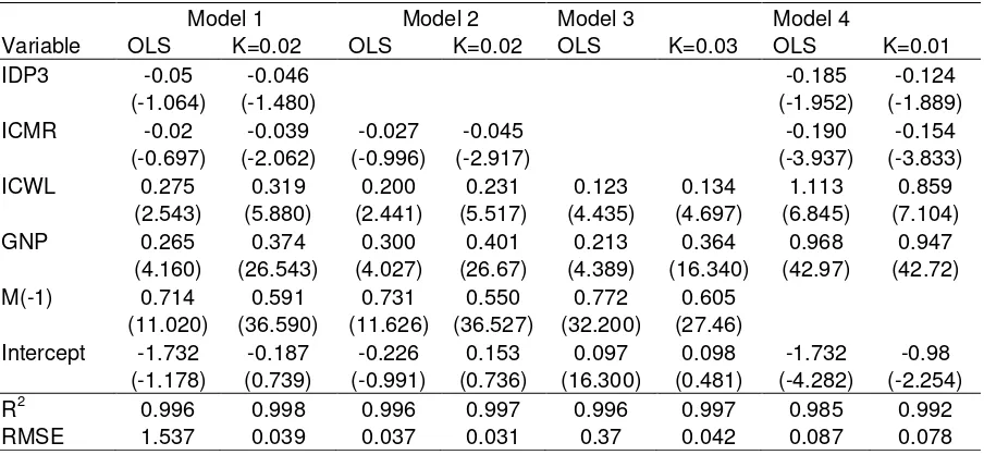
Table 2

Estimated Coefficients and T-values

Model 1 Model 2 Model 3 Model 4

Variable OLS K=0.02 OLS K=0.02 OLS K=0.03 OLS K=0.01

IDP3 -0.05 -0.046 -0.185 -0.124

(-1.064) (-1.480) (-1.952) (-1.889)

ICMR -0.02 -0.039 -0.027 -0.045 -0.190 -0.154

(-0.697) (-2.062) (-0.996) (-2.917) (-3.937) (-3.833) ICWL 0.275 0.319 0.200 0.231 0.123 0.134 1.113 0.859

(2.543) (5.880) (2.441) (5.517) (4.435) (4.697) (6.845) (7.104) GNP 0.265 0.374 0.300 0.401 0.213 0.364 0.968 0.947

(4.160) (26.543) (4.027) (26.67) (4.389) (16.340) (42.97) (42.72) M(-1) 0.714 0.591 0.731 0.550 0.772 0.605

(11.020) (36.590) (11.626) (36.527) (32.200) (27.46)

(6)

Dependent Variable : Real M1 Plus Time Deposit

Independent Variables:

GNP : Real GNP

IDP3 : Interest Deposits 3 Months

ICMR : Interest Call Money Rate

ICWL : Lending Rate

Table 2 shows that the estimators in the ridge regression dominantly have lower variance than those in the OLS regression. It is indicated by the higher values in the ridge regression than the t-values in the OLS except model 4 which dropped Mt-1. RMSE results prove that ridge regression can be better predictor than OLS in the presence of multicollinearity. In all cases, RMSE results of ridge regression are lower than OLS results.

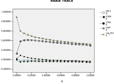
Figure 1. Relationship Between Beta Coefficients and k Value

Figure 1 shows a representative ridge trace for model 1. The Trace shows the path of each coefficient as k increase. The ridge trace clearly shows one aspect of multicollinearity problem. When two independent variables are highly correlated the sum of respective coefficients is likely have a lower variance than either individual coefficients. This is reflected in the traces for GNP and Mt-1 or between interest rate. At levels of k near zero coefficients move in opposite directions revealing a fairly constant sum. The procedure in finding an optimal k from the ridge trace is to search values of k greater than zero until the major instabilities of the coefficients have disappeared.

(7)

Table 3

Wald Coefficient Test

Variable Model 1 Model 2 Model 3 Model 4

IDP3

F-stat = 0.008 Do not reject Ho

ICMR

ICWL

GNP

F-stat = 9.253 Reject Ho

M(-1)

F-stat = 3,652 Do not reject Ho

Where : Ho : i = j

i = beta coefficients from OLS results

j = beta coefficients from Ridge regression

Significance level = 5%

From table 3, it can be seen that in model 1 and model 4, all coefficients of the ridge regression are statistically not different to OLS results. Model 2 and model 3 with lower predictors have one and two estimated coefficients respectively that are different statistically with OLS results. Consistent with Faden (1978), this research found that ridge regression proved superior to OLS regression when the ratio of predictors (p) to sample size (n) or the p/n ratio is high. The bias between ridge estimation and OLS seems disappear when ratio p/n ratio increases. Rozeboom (1979) demonstrated that ridge regression may enhance prediction if the conditions are right. but if not, decreased accuracy would result. These conditions are: a) when there is a high degree of multicollinearity, which was the case here, b) when the samples on which the equations are based are small, and c) when the ratio of p/n is relatively large (Darlington, 1979; Dempster, Schatzoff, & Wermuth, 1977; Faden,1978).

V. Conclusion

(8)

References

Brown, William G, Bruce R. Beattie (1975), Improving Estimates of Economic Parameters by Use of the Ridge Regression With Production Function Applications, American Journal of Agricultural Economics, Vol. 57 No. 1 pp. 21-32

Darlington, R. B. (1978). Reduced variance regression. Psychological Bulletin, 85, 1238-1255.

Dempster, A. P., Schatzoff, M., & Wermuth, N. (1977). A simulation study of alternatives to ordinary least squares. Journal of the American Statistical Association, 72, 77-91,

Faden, V. B. (1978). Shrinkage in ridge regression and ordinary least squares multiple regression estimators. Unpublished doctoral dissertation, University of-Maryland.

Farver, A. S., Sedlacek, W. E., Brooks, Jr., G. C. (1975). Longitudinal predictions of university grades for black and whites. Measurement and Evaluation in Guidance, 7, 243-250.

Grob, J. (2003), Linear Regression, Lecture Notes in Statistics, Springer Verlag

Gujarati, Damodar (2003), Basic Econometrics, Prentice Hall

Hoerl, A. E. & Kennard, R. W. (1970). Ridge regression: Biased estimation for nonorthogonal problems. Technometrics, 12, 69-82,

Price, B. (1977). Ridge regression: Applications to nonexperimental data. Psychological Bulletin, 84, 759-766.

(9)

Rozeboom, W. W. (1979). Ridge regression: Bonanza or beguilement? Psychological Bulletin, 86, 242-249.

Sedlacek, W. E. & Brooks, Jr., G. C. (1976). Racism in American education: A model for change. Chicago: Nelson-Hall..

Tracey, T. J., & Sedlacek, W. E. (in press). Noncognitive variables in predicting academic success by race. Measurement and Evaluation in Guidance.

Tracey, T. J., Sedlacek, W. E., & Miars, R. D. (1983). Applying ridge regression to admissions data by race and sex. College and University, 58, 313-318.