INVERSE MATE
PREDICTION BA
SPHERICAL IND
Ir. I Nyoman Bud
ERIALS PROPERTIES
BASE ON THE VICKER
DENTATIONS
udiarsa, MT, Ph.D
Teknik
Fakultas
Universitas U
ES
ERS AND
INVERSE MATERIALS PROPERTIES
PREDICTION BASE ON THE VICKERS
AND SPHERICAL INDENTATIONS
OLEH
IR. I NYOMAN BUDIARSA, MT, Ph.D
NIP 196602221991031002
TEKNIK MESIN
FAKULTAS TEKNIK
UNIVERSITAS UDAYANA
Contents
1. Introduction 1
2. Mechanical integrity of welded joints and methods in
characterising material constitutive parameters 3
2.1. Spot Welding Process 3 2.2. Effects of Welding parameters on Weld quality 3 2.3. Typical applications and materials system in resistance
Spot welding. 4 2.4. Microstructure and phase transformations during welding 4
2.5. Mechanical integrity of welded joints 5
2.6. The Materials behaviour of metallic materials and
the properties of different welded zones 6 2.7. Mixed experimental and numerical methods in
characterising material constitutive parameters 12 3. Inverse Materials properties prediction base on the Vickers
and spherical indentations. 20
3.1. Introduction and structure of the research work 20 3.2. FE modelling of the Vickers indentation and
effects of material properties 22
3.3. FE modelling of the Spherical indentation and
Effects of material properties 23
3.4. Method to predict material properties from
the Vickers and Spherical indentation 24
3.4.1. Curvature of the Indentation curve 24
3.4.2. 3-D Mapping approach 25
3.4.3. Dimensional analysis and results 26
3.4.4. Chart based Intersection approach and results 28 4. Mechanical testing and FE Modelling of spot welded Joint 45 4.1.Tensile test of the base material and spot welded joint 45 4.2. Drop mass impact test and results 46 4.3. FE modelling of the spot welded joint (Preliminary results) 47
References 57
1.
Introduction
This report is concerned with a analysis on the development of an inverse/reverse
modelling approach to characterise the plastic parameters of elasto plastic materials based
on the indentation method and use the approach to measure the properties of resistance spot welded joints with different material systems. Main objective is:
• To develop an reverse/reverse program to predict the materials properties of elasto plastic materials based on the indentation loading curves and conventional static
hardness measurements;
• To inversely measure the material properties of the nugget, HAZ and base metal zones using indentation methods;
• To develop numerical models with realistic dimensional data, material properties and correlate the modelling results with experimental test results of static and dynamic
deformation;
• To establish the effects of welding parameters on the microstructure (e.g. the dimension of the nugget and heat affected zone (HAZ)) and strength of spot-welded
joints of mild steel and stainless steels (dissimilarmaterials).
Progress to date of both experimental and numerical work is reported, which has met the first three
main objectives of the project. FE models of sharp indenter (Vickers) and blunt indenter
(Spherical indenter) were developed. The effect of some key modelling parameters such as
mesh sensitivity, sample size and boundary conditions were assessed. Three
reverse/inverse modelling methods (designated as dimensional analysis, 3D mapping and
dual indenter chart approach) have been proposed and the validity and accuracy of each
approach in predicting the material properties were systematically evaluated using
numerical indentation curves. In the experimental part, tensile shear tests have been
perform on spot welded joints of different materials. A new drop weight impact testing
method has been developed and a detailed analysis approach has been established and
validated, before used to analyse the performance of spot welded joints of dissimilar
2.
Mechanical Integrity of Welded Joints and
Methods In Characterising Material Constitutive
Parameters
2.1. Spot Welding Process
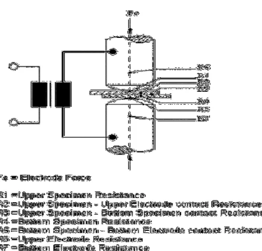
In a spot welding process (Fig. 2.1), two or three overlapped or stacked components are
welded together as a result of the heat created by the electrical resistance, which is
provided by the work- pieces as they are held together under pressure between two
electrodes. As shown in the figure, the secondary circuit of a resistance welding machine
and the work- piece being welded constitute a series of resistances (Aslanlar S., 2006).
The overall resistance also varies with material and the sheet thickness. The force applied
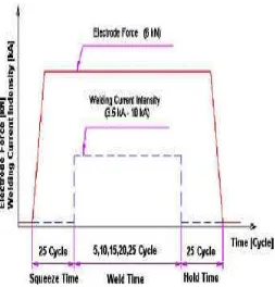
to the electrodes assures its continuity. As illustrated in Fig. 2.2, the sequence of operation
must first develop sufficient heat to raise a confined volume of metal to the molten state.
This metal is then allowed to cool while under pressure until it has adequate strength to
hold the parts together. The current density and pressure must be such that a full nugget is
formed, but not so high causing molten metal being expelled from the weld zone. In
addition, the duration of weld current must be sufficiently short to prevent excessive
heating of the electrode faces The welding process is a complex thermal mechanical
process and the finished assembly consists of regions with significantly different
microstructures and properties, including the base metal, heat affected zone (HAZ) and
weld nugget (Fan X.,2007).
2.2. Effects of welding parameters on weld quality
Weld quality depends on process and material variables that affect the heat generation or
the electrode pressure, among which, the current, force and time are the three main
parameters which determine the strength of the welded joint of a material. The selection of
these three parameters is normally determined by generating a weld lobe as shown in Fig.
2.3. The weld lobe curve is a graphical representation of range of welding variables over
electrode force (Aravinthan, 2003). It is determined by making spot welds using different
combinations of weld time and welding current. Only welds made with currents and weld
times lying within the lobe area are acceptable. Welds made with currents and times
exceeding the upper curve experience expulsion; while welds made with currents and
times below the lower curve are of insufficient size, or no weld is formed. In both cases,
the weld is not acceptable (Aslanlar, et al, 2008).
2.3. Typical applications and materials systems in resistance spot welding
Because of spot welding processes requires relatively simple equipment; it can be easily
converted into an automated operation. Once the welding parameters is established, it
should be possible to produce repeatable welds. The resistance spot welding is the most
widely used joining process for sheet materials. The process is used in preference to
mechanical fasteners, such as rivets or screws, when disassembly for maintenance is not
required (Chou, 2003). The process is used extensively for joining low carbon steel
components for the bodies and chassis of automobiles, trucks, trailers, buses, mobile
homes, motor homes and recreational vehicles and roils road passenger cars, as well as
cabinets, office furniture, and white-goods manufacturing industries (Hasanbasoglu A., et
al, 2007). It is most widely used in joining process for the fabrication of sheet formed
components, with or without requirement of special technique (Vural, 2004). Many
metallic material such as mild steel, high strength steel, galvanized interstitial free steel,
stainless steel, austenitic stainless steel, nickel, aluminium, titanium alloy and brass can be
welded by resistance spot welding (Jou M., 2003; Vural M., et al, 2006; Kahraman N.,
2007). Small scale resistance spot welding (SSRSW) is also one of the main
micro-joining processes being employed in the fabrication of electronic components and devices
to joint thin sheet metals of thickness less than 0.2-0.5 mm (Chang B. H., et al, 2003).
2.4 Microstructure and phase transformations during welding
As described in the sections above, spot welding involves thermal, metallurgical and
mechanical processes, which result in a structure of mixed phases and properties. Fig. 2.4
shows a typical cross-section of spot welded joint of a low carbon steel (Bayraktar, 2004).
There are three main different regions – the base material, the nugget and the
bainitic phases (Ni K, et al, 2004). The region around the nugget, the so-called
heat-affected zone (HAZ), has a mixed microstructure consisting of martensite, bainite, ferrite
and pearlite. The nugget is much harder than the base material due to the quenching effect,
while the HAZ has a gradient mechanical property and a mixed microstructure with the
strength decreasing from the nugget to the base. In many cases, failures of spot welded
joints tend to occur around this region, specifically around the heat-affected zone (HAZ)
(MukhopadhyayM., 2009).
Many research has been conducted to improve the understanding on spot welded joint as
the interactions between electrical, thermal, metallurgical and mechanical phenomena.
(Hou Z., et al, 2006). One active research field is on the prediction of the dimension of
spot welded joints by simulating the welding process with the finite element modelling
(Emmanuel H., et al, 2007; Rahman M. M., et al, 2008). Another active research field is
on the study of microstructure development (Sun D.Q., et al, 2007; Bakavos D.,et al,
2010). The microstructure models have to consider the thermo-physical properties of the
materials in order to describe the phase transformations during heating and cooling stages
(Jou M.,2003, Tan J.C., et al, 2007, Chigurupati P., 2010). These works have resulted in
several models to describe the simultaneous formation that has made it possible to predict
the microstructure development and transformations during spot welding process, and also
to investigate the characteristics and behavior of materials, relating with the applied load
conditions on the spot weld joint
2.5. Mechanical integrity of welded joints
Spot welded joints are widely used in many loads bearing situations and their mechanical
strength has a strong influence on the integrity of the whole structure. A large amount of
research works have been conducted to study the deformation of spot welded joints,
experimentally or numerically, under different loading, such as tensile, bending, impact
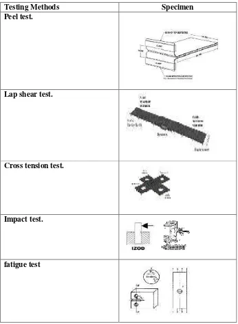
etc. (Darwish, 2003, Cavalli et al, 2003, Yang et al, 2005). Figure 2.5. shows typical
mechanical testing methods of spot welded joint, including peel test, lap shear test,
cross-tension tests, Impact test, corrosion fatique test, and stress corrosion cracking tests
(Alenius, 2006). Each test has its own objectives and the selection of tests hsould be
2.6 The materials behaviours of metallic materials and the properties of different
welded zones
The plastic behaviour is normally described by the constitutive material equations. In
many cases, the three parameter power law hardening rule (Eq. 2.1) is used for steels:
= + ( 2.1)
where the parameter ‘
σ
0’ is the yield stress, ‘K’ is the strength coefficient and ‘n’ is thestrain hardening exponent. These material parameters influence both the yielding strength
and work hardening behaviour of the spot welded joint. The engineering measures of
stress and strain, denoted as and respectively, are determined from the measured
the load and deflection using the original specimen cross-sectional area and length
as
= ; = (2.2)
In the elastic portion of the curve, many materials obey Hooke’s law, so that stress is
proportional to strain with the constant of proportionality being the modulus of elasticity
or Young’s modulus, denoted E:
= (2.3)
Using the true stress = P/A rather than the engineering stress = ⁄ can give a
more direct measure of the material’s response in the plastic flow range. A measure of
strain often used in conjunction with the true stress takes the increment of strain to be the
incremental increase in displacement dL divided by the current length L:
= = = ln (2.4)
This is called the “true” or “logarithmic” strain. During yield and the plastic-flow regime
are offset by decreases in cross-sectional area. Prior to necking, when the strain is still
uniform along the specimen length, this volume constraint can be written:
= 0 = = (2.5)
The ratio is the extension ratio, denoted as λ. Using these relations, it is easy to develop
relations between true and engineering measures of tensile stress and strain
= 1 + = .λ
= ln 1 + = "#λ (2.6)
These equations can be used to derive the true stress-strain curve from the engineering
curve.
The failure of spot welded joints can be overload failure and fracture (Lee H., et al, 2005).
Fracture is separation, or fragmentation of a solid body into two or more parts under the
action of stress. Fractures of metals are classified two sorts as the fracture behaviour:
brittle fracture and ductile fracture. The ductile fracture process in metals usually follows
a sequence of three stages: (a) Formation of a free surface at an inclusion or second phase
particle by either interface decohesion or particle cracking, (b) Growth of the void around
the particle, by means of plastic strain and hydrostatic stress, (c) Coalescence of the
growing void with adjacent voids. The linking of voids may occur on planes which are
perpendicular to the applied stress (normal rupture), or are parallel to it (delimitation), or
along shear bands at angle to it (shear fracture). Most attempts at understanding ductile
fracture have considered only the first type. Once a microvoid has been nucleated in a
plastically deformed matrix, by either the bending or cracking of a second-phase particles
or inclusions, the resulting stress-free surface of the void causes localized stress and strain
concentration of the adjacent plastic field. The fracture of spot welded joints is a ductile
fracture.
Gurson model is widely used in ductile fracture mechanics, in which, the fracture of
material is considered as the result of void growths in the material volume. The
Homogenous material surrounding the void is called matrix material. The Gurson model
can realistically represent failure, provided the loading state in the coupon used to
determine the Gurson parameters, is similar to that in the rupture zone of the structure.
Gurson-Tvergaard-Needleman (GTN) model (ABAQUS Theory Manual 6.9), which is briefly described
below. The original model developed by Gurson, assumed plastic yielding of a porous
ductile material, where the yield surface was a function of a spherical void as follows
$ = %&'(&'(
)*+,) + )- ./01 %*2
)*+, − 4 +
-) = 5 ( 2.7)
Where 6 is the yield stress of the material, 7 is the mean stress, 8 is the void volume
fraction. 8 = 0 implies that the material is fully dense, and the Gurson yield condition
reduces to that of von Mises; 8 = 1 implies that the material is fully voided and has no
stress carrying capacity. 9:; is the components of stress deviator ( <, > = 1, 2,3 , defined
as
&'(= *'(− *2 A'( ( 2.8)
And B:; is the Kronecher delta
A'(= C4 ' = ( 5 ' ≠ (E
Theoretical micromechanical studies for materials containing periodic distribution of
cylindrical or spherical voids have been carried out by Tvergaard (2000). By considering
the influence of neighbouring voids on each pair of voids, three parameters, q1, q2, q3,
have been added to equation ( 2.9)
$ = %&'(&'(
)*+,) + ) F4 - ./01 % F) *2
) *+, − 4 + F%
-) = 5 ( 2.9)
G1, G2, G3 are material constants and it was found that matching of test results can be achieved for most alloys, by taking the following material values (ABAQUS Theory
Manual 6.4):
Tvergaard and Needleman have further modified the Gurson model by replacing 8 with an
effective void volume fraction, 8∗ 8 :
-∗= L
- '- - ≤ -N
-N+ -PPPPQ--OOQ-NN - − -N
-O
PPP '- - ≥ -O
E '- -N < - < -O ( 2.10)
Where :
-O
PPP = F4+ TF4)− F%
F%
The parameter 8U and 8V model the material failure due to mechanisms such as micro
fracture and void coalescence. 8U is a critical value of the void volume fraction, and 8V is
the value of void volume fraction at which there is a complete loss stress carrying capacity
in the material
The total charge in void volume fraction is given as
-W = -WXY+ -WZ[N\ (2.11)
Where 8W]^is charge due to growth of existing voids and 8W_`U is change due to nucleation
of new voids. Growth of the existing voids is based on the law of conservation of mass
and is expressed in terms of the void volume fraction
-XYW = 4 − - aW.b\∶ d
e:; = B:; the unit second order tensor
The nucleation of voids is given by a strain-controlled relationship:
-WZ[N\ = f aPW2b\
Where
f =
-Z&g√) i
jkl m−
4 )
n
aP2b\Q ag
&g
o
)
The normal distribution of the nucleation strain has a mean value q and standard
deviation 9q, 8_ is the volume fraction of the nucleated voids. Gurson model has been
implemented in several FE modelling software, like ABAGUS, ADINA, SYSTUS, etc,
and is widely used by researchers (ABAQUS Theory Manual 6.9)
Fatigue failure is another problem associated with spot welded joints. Fatigue is the
progressive and localized structural damage that occurs when a material is subjected to
cyclic loading. The maximum stress values are less than the ultimate tensile stress limit,
and may be below the yield stress limit of the material. Some common fatigue
mechanisms on metallic material include Time-varying Loading fatigue, Thermal fatigue,
Corrosion Fatigue, Surface/Contact Fatigue, combined creep and Fatigue (Matos A.,
2010) Time-varying loading fatigue can be defined as a process caused by time-varying
load which never reach a high enough level to cause failure in a single application, and yet
results in progressive localized permanent damages on the material. The damages, usually
cracks, initiate and propagate in regions where the strain is most severe. When the local
damages grow out of control, a sudden fracture/rupture ends the service life of the
structure. Common categories and approaching methods, include:
The S-N curve Stress Life Method, is the basic method presenting fatigue failure in high
cycles (N > 105) which implies the stress level is relatively low and the deformation is in
elastic range. Users may check the maximum and minimum stress directly. Define R is the
ratio of minimum stress to the maximum stress. Alternatively, define A is the ratio of
alternating stress to mean stress.
r = stuv
stwx (2.13)
= sw
st=
Qy
zy (2.14)
An approximation based on the zero-mean stress S-N curve proposed by Goodman and Gerber is written as
{ = | }1 − }sst~• 6
Where
| is the stress at fatigue fracture when the material under zero mean stress cycled
loading
7 is the mean stress of the actual loading.
` is the tensile strength of the material
R = 1 is called Goodman line which is close to the results of notched specimens.
r = 2 is the Gerber parabola which better represents ductile metals.
Individual contributions, known as Palmgren-Miner's linear damage hypothesis or Miner's
rule.
∑
_u •uqu •u
‚
:ƒ
= „
(2.16)
Where
k is the total number of different stress magnitudes in a spectrum
9:(1≤ < ≤ …) is the magnitudes of each different stress in sprectrum
#: 9: is the actual number of cycle under the specific stress 9:
†: 9: is the total number of cycle to failure under the specific stress 9: 0.7 < c < 2.2 is an material dependent constant obtained by experiments.
Set c = 1, if there is no further information available
Derived relationship for the stage II crack growth with cycle N, in term of the cyclical
component ∆K of the stress intensity factor K
{
q
= ‡ ∆
7 (2.17)Where ‰ †⁄ is the crack length and m is typically in the range 3 to 5 (for metal)
The impact strength of spot welds is a very important quality index in the automotive
industry, impact test conducted to determine the impact energy & Impact performance of
weld through impact process characteristics such as impact force and displacement
profiles (Zhang H., et al, 2001). Impact tests were also performed to evaluate of resistance
to dynamic failure in the characteristics and behaviour of thin welds of different grades of
determined by integration of the force vs. deformation curve. The mean crush load for a
given deformation is defined as the absorbed energy divided by the deformation
The energy absorbed by the specimen during crushing, EA, is equal to the area beneath the
load vs. displacement curve and can be defined as follows (Joosten M.W., 2010):
EA =
"
(2.18)where " is the stroke or displacement of the crosshead and is the applied axial force. The
specific energy absorption, SEA, is defined as the energy absorbed per unit mass of
destroyed structure and can be defined as follows:
SEA = 9‘•’„‘’•Ž “Ž<•ℎ‘Š‹Œ•ŠŽ #Ž•••
SEA = •–
—
(2.19)
which is a function of the density, ˜, the cross sectional area of the structure, A, and the
absorbed energy, EA, over a crushing stroke, ". Note that the cross sectional area in the
steeple trigger zone is not constant, and is calculated as a function of the axial
displacement,".
On axial crushing test with high speed crushing, the value of impact energy similar with
that given in eq.2.20
EA = I › œI (2.20)
Where m is the mass of the crosshead and v the crush velocity
2.7. Mixed experimental and numerical methods in characterising material constitutive parameters
The elastic-plastic material parameters and the fracture parameters of materials can be
readily determined when standard specimens are available. However, for a spot welded
joint, standard testing is not applicable to characterise the HAZ and nugget due to their
to use a mixed experimental-numerical method based on the indentation test to inversely
characterise the parameters of the constitutive material laws for the nugget, HAZ and the
base. In a mixed numerical-experimental approach, the load-deformation data of the
material is used as input data to a finite element (FE) model that simulate the geometry
and boundary conditions of the experiment. This approach has been used on some
non-standard specimens or surface loading situations, such as in vivo (within a living
organism) tension, indentation, etc. (Meuwissen et al, 1998, Shan et al, 2003; Gu et al,
2003; Bolzon et al, 2004, Ren et al, 2006). With indentation tests, the local plastic
properties can be calculated by solving the inverse problem via finite element analysis by
incrementally varying properties in 3D modeling to find a similar simulated load–
displacement curve as compared with experimental one.
Fig. 2.1 The setup of a spot welding system and the resistances occurring in the welding
Fig. 2.2 Basic welding cycle(s) for spot welding (Aslanlar S., 2006).
(a) Different structure zone of steel weldment (Bayraktar E., 2004)
(b) Typical structure of welded joint of dissimilar materials, A- Asymmetric penetration in the dissimilar metal joint of EN 1.4318 2B and ZStE260BH steels; B - dissimilar metal joint of EN 1.4318 2H and DX54DZ steels (Alenius, 2006)
Fig. 2.4 Different structure zones of welded joints.
Base Nugget Heat affected zone
(HAZ)
Grain
growth zone
Recrysatllised
zone
Partial
transformed zone
Tempered
zone
Testing Methods Specimen Peel test.
Lap shear test.
Cross tension test.
Impact test.
fatigue test
(a)Different types of indenters
(b)
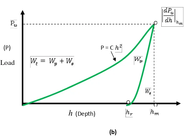
Figure. 2.6 (a) Different indenter types; (b) Schematic illustration of a typical P-h
response of an elasto plastic material to sharp indentation
P = C (P)
Load
Fig. 2.7 Parametric modelling approach to extract the material properties(Ren et al 2006).
3.
Inverse Material Properties Prediction Base On
The Vickers And Spherical Indentations
3.1. Introduction and structure of the research work
The deformation of spot welded joints is challenging research problem due to the complex
nature of the structure. One major problem is to characterise the materials properties. The
elastic-plastic material parameters and the fracture parameters of materials can be readily
determined when standard specimens are available. However, for a spot welded joint,
standard testing is not applicable to characterize the HAZ and nugget due to their complex
structure and small size. In an previous work, an parametric based approach has been
developed, which determine the material parameters by cross compare an indentation
curve with numerical curves for all the materials properties over a wide spectrum, then
using the objective functions the mean to determine the final optimum data (Kong, 2008).
This has opened up the possibility to characterize the material properties based a dual
indenter method. However, the method involved intensive data fitting which has to be
performed based on a computational program. This work aims to further develop this
method based to enable more direct parameter prediction based on analytical or
semi-analytical approaches with either continuous indentation loading curve or conventional
hardness tests. The approach will then be used to test different welding zones and the
material parameters thus predicted used to simulate the deformation of spot welded joints
under complex loading conditions including tensile shear and drop weight impact tests.
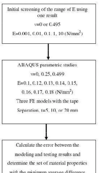
Figure 3.1 shows the work plan of the project. In the first stage FE models of sharp
indenter (Vickers) and blunt indenter (Spherical indenter) were developed. The effect of
some key modelling parameters such as mesh sensitivity, sample size and boundary
conditions were assessed. The accuracy of the Vickers indentation was validated by
comparing the modelling results with published data. In the next stage, the effect of the
key material properties including the work hardening coefficient and the yield strength
analysis, 3D mapping and dual indenter chart approach) have been proposed and the
validity and accuracy of each approach in predicting the material properties were
systematically evaluated using numerical indentation curves. In the experimental part,
tensile shear tests have been perform on spot welded joints of different materials. A new
drop weight impact testing method has been developed and a detailed analysis approach
has been developed and validated, before used to analyse the performance of spot welded
joints of dissimilar materials In the next stage, the inverse material properties approach is
to be extended to conventional hardness tests to characterise the properties of different
structure zones within the welded joints. The properties predicted will then be used to
develop a numerical model with realistic material poverties to simulate the deformation of
the joint under different loading conditions.
Commercial finite element analysis (FEA) software package ABAQUS version 6.9.1 is
used in the numerical simulation. The elastic-plastic materials behaviours were
represented, respectively, by Hooke’s law and Von Misses yield criterion with isotropic
power law hardening. In the models, the true stress-strain behaviour of the materials
following constitutive law
= •
r
8Œ• ≤
_8Υ >
66
E
(3.1)
Where is the Young’s modulus, r a strength coefficient, n the strain hardening
exponent and 6 the initial yield stress at zero offset strain. In the plastic region, true strain
can be decomposed to strain at yield and true plastic strain
=
6+
Ÿ(3.2)
For continuity at yielding, the following condition must hold ( = 6 )
If the yield stress ( 6) is defined at zero offset strain. Hence the true stress-true strain
behaviour is written to be (Swaddiwudhipong et al, 2005):
=
,
6
n
s¡¢o
__
E
(3.4)
In these indentation FE models, the Young’s modulus ‘E’ of the work piece materials was
set to 200 GPa and Poisson’s ratio was set to 0.3, which were commonly used value for
steel (Chen et al, 2007).
3.2. FE modelling of the Vickers indentation and effects of material properties
Figure 3.2.(a) show the FE Models of the Vickers indentation. Only a quarter of the
indenter and material column was simulated as a result of plan symmetric geometry. The
sample size is more than 10 time the maximum indentation depth, which is sufficiently
large to avoid any sample size effect or boundary effect (Johnson, 1985). The bottom face
of the material volume was fixed in all degrees of freedom (DOF) and two side faces (A
and B) were symmetrically fixed in z and x direction. The element type used is C3D8R
(reduced integration element used in stress/displacement analysis). Contact was defined at
indenter facet. The material of interest was allowed to move and the contact between the
indenter surface and the material was maintained at all the time. The mesh in the regions
with large deformation such as that directly under the indenter tip was refined with high
mesh density in order to obtain more accurate results.
The Vickers indenter has the form of the right pyramid with a square base and an angle of
136 between opposite face. It is normally made of diamond with Young’s modulus of over 1000 GPa, which is significantly stiffer than steel (E=200 GPa). The indenter was
considered as the rigid body to improve the modelling efficiency. A predefined
displacement was applied in a ramp mode and the reaction force is recorded on the
reference point, representing the overall load on the indenter. Figure 3.2 (b) shows a
typical P-h curve (Force Vs Indentation depth) during loading and unloading phase ( 6
penetration, while difference between the loading and loading curve represents the energy
loss (Swaddiudhipong et al, 2005). The unloading part of the P-h curve is primarily
influenced by E, as it is essentially an elastic process, while the loading part of the P-h
curve correlates with 6 and n (Taljat, 1998). This work is focused on the studies of
plastic parameters, so only the loading curve was utilised to predict the plastic material
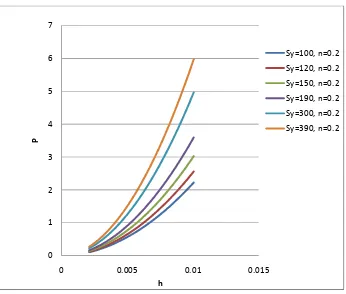
parameters. Figure 3.3 (b) illustrated the effect of material properties on the P-h curves of
Vickers indentation ( 6 =300 MPa) with E set at 200 GPa for Steel. It is clearly shown
that both the yield strength and work hardening coefficient influence the indentation
curves.
3.3. FE modelling of the spherical Indentation and effects of material properties
Different from the Vickers indenters, spherical indenter is fully asymmetric, a typical FE
model is shown in Figure.3.4.(a). A planar specimen (3X3››I) has been used and this
specimen size is large enough to avoid potential sample size effect. The movement of the
indenter was simulated by displacing a rigid arc (rigid body) along the Z axis. The bottom
line was fixed in all degree of freedoms (DOF) and the central line was symmetrically
constrained. The element types used in the spherical indentation model are CAX4R and
CAX3 (4-node bilinear asymmetric quadrilateral and 3-node linear asymmetric triangle
element used in stress/ displacement analysis without twist).
A gradient meshing scheme has been developed for different regions. The mesh size is
5¤m in the region underneath and around the indenter as shown in Figure 3.4.(b), while
the mesh size of other regions from the nearest region to the outer edge varied from
10 ¤m, 0.05 mm and 0.1mm; the mesh of the transitional regions is mainly triangle
element following a free meshing scheme. Figure 3.4 (c) shows a typical numerical force
indentation depth curve (loading and unloading curves) of a spherical indenter (R= 0.5mm
6= 500, n=0.024). The curve is significantly different from Vickers with much higher
forces due to the larger contact area in a spherical indentation. Figure 3.5 illustrate the
effect of plastic material properties on the P-h curves of the Spherical indentation. It
clearly shows that both the yield stress and work hardening coefficient influence the
3.4. Method to predict material properties from the Vickers and spherical indentation
3.4.1. Curvature of the indentation curve
As shown in Figures 3.3-5, the P-h curves for both Vickers and Spherical indentation obtained the following relationship:
C =P ℎ⁄ I (3.5)
Where P and are the load and indentation depth on the loading curve respectively. C is
the curvature coefficient with the curvature for the Vickers Indentation and spherical
indenter designated as ‡¦ and ‡§ respectively. The curvature is a function of the yields
stress and the work hardening coefficient. This will provide a relationship which potential
allow the prediction of material parameters from continuous indentation tests.
Figure 3.6 is a flow chart showing the main structure of the inverse modelling approach to
predict the material properties. In the first stage, systemic FE models were developed to
form he simulation space covers the potential range of material properties. In the next
stage, the loading curves were used to develop an simulation space. The data will then be
processed through three different approaches (3D mapping, dimensional analyse, and dual
indenter chart approach) to predict the material parameters. Details of each approach and
the results were presented in the next sections with discussion.
The three approaches have been comparative developed to assess their suitability to
predict the materials properties based on the dual indenter approach. The second approach
is normalised dimensionless analysis in which the relationship is normalised than a
dimensionless analysis is applied. In the third approach, the relationship between the
curvature for both the Vickers and spherical were developed then used a chart to predict
all the material sets with the same curvature. The relationship is used to predict the
material sets have the sane indentation curvature. The key procedures of each approach
and the typical results are detailed in the next three sections.
3.4.2. 3D- Mapping approach
In the 3D mapping approach, the curvature data were plotted against the materials
properties, the an equation is developed base on either linear or nonlinear fitting, which
will give an equation between curvature and working hardening and yield stress.
illustrated by the surface show Figure 3.7. The data for construction of these surfaces
were obtained numerically through indentation finite element analysis encompassing a
domain of 6 from 100 to 190MPa and n varying from 0.01 to 0.5 It clearly showed that
the curvature coefficients increased with 6 and n but with different gradients for different
regions.
The evaluation performed on surface plot 3D of loading curvature and properties material,
this approach was started by setting the value of curvature and properties material as
mapping 3D. A linear fitting plane is shown in Figure 3.7(a) & (b). For each curvature
value, there are an array of material property sets. These data were extracted and plotted in
Figure 3.7 (c). The material property set at the intersection point between the data for the
Vickers and Spherical indentation will represent the true material properties. The
accuracy of the approach has been assessed using a range of initial values, the results were
listed din Table 3.1. Similar approach has been applied to the data using Nonlinear
(Parabolic) mapping and the results were shown in Figure 3.8 (a)(b) and the results of the
accuracy test was listed in Table 3.2.
Evaluation of accuracy on the approach using 3D chat mapping carry out by taking input
data which is characterized by randomize and represent the sample space. The selected
input data with 2 variations in the value (n), namely n=0.15 and n=0.28 (range 0.01 0.30)
and 6 = 100, 140, 190 and 300. Accuracy study chat mapping 3D-Linier (Table.3.1),
known that on average value of different predictive of (n) into n-input as n=0.056
0.069 and average accuracy error ∆n n⁄ (%) is 0.1% both the prediction (n) on Vickers
Indentation and on Spherical Indentation. This shows the selected predictors significantly
acceptable within the limit of level confidence less than 0.5 %. While on an Accuracy
study chat mapping 3D-Non Linier (parabolic) (Table.3.2.), known that on average value
of different predictive of (n) into n-input as n=0.059 0.061 and average accuracy error
∆n n⁄ (%) is 0.22% both the prediction (n) on Vickers Indentation and on Spherical Indentation. This shows the selected predictors significantly acceptable within the limit of
level confidence less than 0.5 %. By Comparing the two approaches chat mapping 3D,
known to have smaller average error by prediction using mapping 3D linear ∆n n⁄ (%) is
0.1% compared using the non linear (parabolic) ∆n n⁄ (%) is 0.22%. This evaluation
showed that the 3D chat mapping approach can serve as predictor value work hardening
coefficient (n) of both the prediction (n) on Vickers Indentation and on Spherical
3.4.3. Dimensional analysis and results
In the dimensional analysis, an relationship between the curvature the material properties
were developed based on the dimensional analysis. Dimensional analysis has proven to be
useful to the study of the contact mechanics for instrumented normal indentation (Cheng.
et al, 2004). In Indentation, indenting normally into a power law elasto plastic solid, the
load P can be written as (Dao, 2001).
P = P h, E, v, Eª, vª, σ¬, n (3.6)
Where Eª is Young’s modulus of the indenter, and vª is its Poisson’s ratio. By combining
elasticity effects of an elastic indenter and an elasto plastic solid as
P = P h, E∗, σ
¬, n (3.7)
Where
E
∗= }
Q-®•
+
Q-u®•u
•
Q
(3.8)
Alternatively, equation (3.7) can be written as
P = P h, E∗, σ
¯, n (3.9) Or
P = P h, E∗, σ
¬, σ¯ (3.10)
Applying the theorem in dimensional analysis, equation (3.9) becomes
P = σ° hI ∏ 1 • ∗
²³, n (3.11)
C = ¶µ®= σ¯∏ 1 ·• ∗
²³, n¸ (3.12)
Where ∏ 1 is a dimensionless function. similarly, applying the theorem to equation
(3.10), loading curvature C may alternatively be expressed as
C = ¶µ®= σ¬ ∏ 1 n• ∗ ²¹ ,
²³
²¹o (3.13)
Where ∏ 1 is a dimensionless function, the dimensionless given in equation (3.12). and
the normalization was taken with respect to E∗ instead of 6 or ^
Figure 3.9.(a) shows the relationship between normalised Cv Vs properties material, and
Figure 3.9.(b). Show the relationship between normalized Cs Vs properties material (strain
hardening exponent (n) and Yielding stress). It is clearly shown that all the data. Curve
fitting has been performed by iterating the relationship between loading curvature
indentation and properties material ( 6, # as following equations
C
-=
6J º⁄374.14 Ž
J. ½¾ _(3.14)
Similarly an equation has been determined for the Spherical indentation
C
¿=
6J º⁄8011.9 Ž
.½Âº _ (3.15)Using the relationship determined, for each combination of Cv and Cs, there are a range of
material data as shown in Figure 3.9.(c). The intersection point will represent the predicted
material properties. In this case, for 6= 150, n=0.2, Cv = 30647.664 and Cs = 515752.
The predicted value are ′6= 149, n’ =0.209.Accuracy studies results were done for some
input value, the results were listed in Table 3.3. The average accuracy error ∆ 6 / 6 =
0.065196 and n/n = -0.06296, which is much better than the accuracy for the 3D
3.4.4. Chart based Intersection approach and results
In the chart based intersection approach, the potential material sets with the same
curvature value for the Vickers and spherical indenters were identify separately through a
chart (C vs. N) for different yield stress (Figure 3.10 (a) & (b)). The property data was
then plotted onto another chart for yield stress vs. Work hardening coefficient (Figure 3.10
c). The properties were determined at the intersection point between the data for the
Vickers and Spherical indenters. As illustrated in Figure 3.10 (a), (b), (c) with a known Cv
or Cs value, the properties can be determined by drawing a straight line along the
curvature value, the intersection point represents data with the same curvature value.
These data was then plotted onto the yield stress-work hardening n chart. The intersection
point will represent the predicted material properties. The two cases represents two
examples for ( 61= 150, n1=0.15) and ( 62= 300, n2=0.28), both are very close to the
true material properties. Prediction carry out by determining the value of n (work
hardening coefficient) based on analysis of trend equations at each curvature Through chat
fitting and mapping knowable predicted value n1 = 0.174 , n2 =0.209 as described on
accuracy study results of inverse FE modeling on Vickers and spherical indentation
plotting and mapping data result. Evaluation of accuracy on the approach using Plotting
and mapping carry out by taking input data which is characterized by randomize and
represent the sample space. The selected input data with 2 variations in the value (n),
namely n=0.15 and n=0.28 (range 0.01 0.30) and 6 = 100, 140, 190 and 300. Accuracy
study Plotting and mapping (Table.3.4), known that on average value of different
predictive of (n) into n-input as n=0.24 and average accuracy error ∆n n⁄ (%) is 0.07%
both the prediction (n) on Vickers Indentation and on Spherical Indentation. This shows
the selected predictors significantly acceptable within the limit of level confidence less
than 0.5 %.Accuracy studies results were done for some input value, the results were listed
in Table 3.4. The average accuracy, which is much better than the accuracy for the 3D
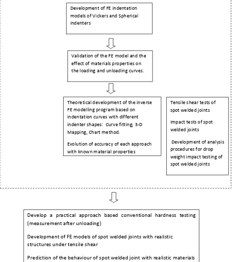
Figure 3.1 Flow chart showing the Research work. Development of FE indentation models of Vickers and Spherical indenters
Validation of the FE model and the effect of materials properties on the loading and unloading curves.
Theoretical development of the inverse FE modelling program based on indentation curves with different indenter shapes: Curve fitting; 3-D Mapping, Chart method.
Evolution of accuracy of each approach with known material properties
Tensile shear tests of spot welded joints
Impact tests of spot welded joints
Development of analysis procedures for drop weight impact testing of spot welded joints
Develop a practical approach based conventional hardness testing (measurement after unloading)
Development of FE models of spot welded joints with realistic structures under tensile shear
(a)
(b)
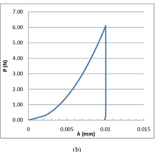
Figure 3.2 (a) FE model of the Vickers Indentation test; (b) Typical force- Indentation depth (P-h) curve during loading and unloading of the Vickers indentation ( 6= 100 MPa, n= 0.01)
0.00 1.00 2.00 3.00 4.00 5.00 6.00 7.00
0 0.005 0.01 0.015
P
(
N
)
h(mm)
A B
136 between
[image:31.612.184.432.382.625.2](a) Effect of the yielding strength
(b) Effect of work hardening coefficient.
Figure 3.3 Effect of work hardening and yield strength on the P-h curves of the Vickers indentation.
0 1 2 3 4 5 6 7
0 0.005 0.01 0.015
P
h
Sy=100, n=0.2 Sy=120, n=0.2 Sy=150, n=0.2 Sy=190, n=0.2 Sy=300, n=0.2 Sy=390, n=0.2
0.000E+00 1.000E+00 2.000E+00 3.000E+00 4.000E+00 5.000E+00 6.000E+00 7.000E+00
0.000E+00 5.000E-03 1.000E-02
P
h
[image:32.612.136.482.62.356.2](a) FE model of the Spherical (b).Close-up view showing the Indentation test the mesh underneath the indenter
Figure.3.4(a), (b) FE models of the Spherical Indentation test (R=0.5mm).
(c)
Figure.3.4.(c). Typical force-indentation depth (p-h) curve during loading and unloading for Spherical Indentation ( 6= 500 MPa, n=0.024).
0 20 40 60 80 100 120 140
0 0.005 0.01 0.015 0.02 0.025
P
(
N
)
Figure 3.5 (a) Effect of yield stress ( 6) as plastic parameter on the p-h curves of the spherical Indentation.
Figure 3.5 (b)Effect of Work hardening coefficient (n) as a plastic parameter on the P-h curves of the spherical indentation
0 20 40 60 80 100
0 0.005 0.01 0.015 0.02 0.025
P
(
N
)
h (mm)
SY=100 n= 0.01 SY=200 n=0.01 SY=300 n=0.01 SY=400 n=0.01 SY=500 n=0.01
0.000E+00 5.000E+00 1.000E+01 1.500E+01 2.000E+01 2.500E+01 3.000E+01 3.500E+01 4.000E+01 4.500E+01 5.000E+01
0.000E+00 5.000E-03 1.000E-02
P
h
Sy 200, n=0.01
Sy 200, n=0.1
Sy 200, n=0.2
[image:34.612.179.437.89.366.2] [image:34.612.176.439.416.654.2]Input experimental Force Vs depth data
[image:35.612.168.436.83.662.2]Simulation Space
Figure 3.6. Flow chart showing the inverse FE modelling approach based on the Vickers and Spherical Indentation tests.
0 50 100
0 0.01 0.02 0.03
P ( N ) h (mm) 0 20 40 60 80 100
0 0.02 0.04
P
(
N
)
h (mm)
0 1000 2000 3000 4000
0 1 2 3
S tr e ss , M p a Strain
Three inverse properties prediction methods:
• Dimensional analysis
approach
• 3D mapping approach • Dual indenter Chart based
*
+and n
[image:36.612.86.504.83.291.2] [image:36.612.103.516.377.638.2]
Figure 3.7 (a).Surface mapping (linear fitting) plot of loading curvature vs material properties.
Figure 3.7 (b). Typical materials parameter prediction process based on linear 3-D mapping method -3.00E-01 -2.00E-01 -1.00E-01 0.00E+00 1.00E-01 2.00E-01 3.00E-01 4.00E-01 5.00E-01 6.00E-01 7.00E-01
0 50 100 150 200 250 300 350
n
Yield Stress, Mpa
Accuracy study
Input data Vickers Indentation + Spherical indentation
Material properties Value curvature Predicted value
Different with input value
Accuracy (error %)
Predicted value
Different with input
value
Accuracy (error %)
n *+ Cv Cs n ∆n ∆n/n n ∆n ∆n/n
0.15 100 26008 466275 2.052E-01 5.523E-02 3.682E-01 2.477E-01 9.770E-02 6.513E-01
0.15 140 26008 466275 1.538E-01 3.786E-03 2.524E-02 1.639E-01 1.388E-02 9.253E-02
0.15 190 26008 466275 8.949E-02 -6.051E-02 -4.034E-01 5.911E-02 -9.089E-02 -6.059E-01
0.15 300 26008 466275 -5.198E-02 -2.020E-01 -1.347E+00 -1.714E-01 -3.214E-01 -2.143E+00
0.28 100 61940 925826 5.749E-01 2.949E-01 1.053E+00 6.391E-01 3.591E-01 1.283E+00
0.28 140 61940 925826 5.235E-01 2.435E-01 8.695E-01 5.553E-01 2.753E-01 9.833E-01
0.28 190 61940 925826 4.592E-01 1.792E-01 6.398E-01 4.506E-01 1.706E-01 6.091E-01
[image:37.792.35.772.135.375.2]0.28 300 61940 925826 3.177E-01 3.770E-02 1.346E-01 2.201E-01 -5.994E-02 -2.141E-01
Table 3.1. Accuracy study results of inverse FE modelling on Vickers and Spherical indentation by 3D Linier Predicted chart mapping
Figure 3.8 (a).Surface mapping (nonlinear fitting) plot of loading curvature vs
material properties.
Figure 3.8 (b) Typical materials parameter prediction process based on nonlinear 3-D mapping method. -6.00E-01 -4.00E-01 -2.00E-01 0.00E+00 2.00E-01 4.00E-01 6.00E-01 8.00E-01
0 100 200 300 400
n
Yield Stress, Mpa
Cv 150 Cv 300 Cs 150 Cs 300 Cs 180 0 2e+4 4e+4 6e+4 8e+4 1e+5 100 120 140 160 180 0.1 0.2 0.3 0.4 C v Sy n 0.0 2.0e+5 4.0e+5 6.0e+5 8.0e+5 1.0e+6 1.2e+6 120 140 160 180 0.1 0.2 0.3 0.4 C s Sy n 3D Non linear
[image:38.612.105.480.80.283.2] [image:38.612.103.490.372.615.2]Table 3.2. Accuracy study results of inverse FE modelling on Vickers and Spherical indentation by 3D Non Linier (Parabolic ) Predicted chart mapping
Accuracy study
Input data Vickers Indentation- Spherical indentation
Material properties Value curvature Predicted value
Different with input value
Accuracy (error %)
Predicted value
Different with input
value
Accuracy (error %)
Sy n *+ Cv Cs n ∆n ∆n/n n ∆n ∆n/n
150 0.15 100 26008 466275 0.230977 8.098E-02 5.398E-01 0.270383 1.204E-01 8.026E-01
150 0.15 140 26008 466275 0.166904 1.690E-02 1.127E-01 0.175556 2.556E-02 1.704E-01
150 0.15 190 26008 466275 0.077722 -7.228E-02 -4.819E-01 0.034696 -1.153E-01 -7.687E-01
150 0.15 300 26008 466275 - - - - - -
300 0.28 100 61940 925826 0.490031 2.100E-01 7.501E-01 0.562677 2.827E-01 1.010E+00
300 0.28 140 61940 925826 0.454171 1.742E-01 6.220E-01 0.505893 2.259E-01 8.068E-01
300 0.28 190 61940 925826 0.412688 1.327E-01 4.739E-01 0.43741 1.574E-01 5.622E-01
300 0.28 300 61940 925826 0.33883 5.883E-02 2.101E-01 0.301386 2.139E-02 7.638E-02
180 0.25 100 61940 925826 0.354054 1.041E-01 4.162E-01 0.399732 1.497E-01 5.989E-01
180 0.25 140 61940 925826 0.30762 5.762E-02 2.305E-01 0.326902 7.690E-02 3.076E-01
180 0.25 190 61940 925826 0.251198 1.198E-03 4.792E-03 0.233276 -1.672E-02 -6.689E-02
Figure 3.9(a) Effects of Yield strength ( 6) on the value loading curvature (Cv) and work hardening coefficient (n) on Vickers Indentation.
Figure 3.9 (b) Effects of Yield strength ( 6) on the value loading curvature (Cs) and work hardening coefficient (n) on Spherical Indentation
y = 374.1e3.196x
0 200 400 600 800 1000 1200 1400 1600
0.000 0.100 0.200 0.300 0.400 0.500
C v /s y ^ 3 /4 n Sy=100 Sy=120 Sy=150 Sy=190 Sy=300 Prediction Cv Expon. (Prediction Cv)
y = 8011.e1.983x
0 5000 10000 15000 20000 25000 30000 35000
0 0.2 0.4 0.6 0.8
[image:40.612.105.486.64.338.2] [image:40.612.106.496.394.674.2]
Figure 3.9(c). Typical materials parameter prediction process based on the intersection between properties line for the Vickers and Spherical indentation ( 6= 120 Mpa, n=0.2).
0.000000E+00 5.000000E+01 1.000000E+02 1.500000E+02 2.000000E+02 2.500000E+02 3.000000E+02
0 0.1 0.2 0.3 0.4 0.5 0.6
Y
ie
ld
t
re
ss
(
M
p
a
)
Work Hardening coefficient (n)
Sy(n,Cv)
[image:41.612.105.491.110.518.2]Input data Accuracy study
Material properties Value of Curvature Predicted values Differences with input value Accuracy (error%)
σy n Cs Cv σy n ∆σy ∆n ∆σy / σy ∆n/n
100 0.1 303841.62 15725.77 102 0.09 -2 0.010 -0.020 0.10000
100 0.2 387159.42 22631.67 105 0.19 -5 0.010 -0.050 0.05000
100 0.3 495483.94 32535.09 111 0.29 -11 0.010 -0.110 0.03333
200 0.1 5.260E05 2.771E+04 202 0.09 -2 0.010 -0.010 0.10000
200 0.2 6.297E05 3.767E+04 195 0.21 5 -0.010 0.025 -0.05000
200 0.3 7.547E05 5.061E+04 195 0.31 5 -0.010 0.025 -0.03333
290 0.1 6.892E05 3.734E+04 275 0.12 15 -0.020 0.052 -0.20000
290 0.2 8.039E05 4.885E+04 265 0.22 25 -0.020 0.086 -0.10000
290 0.3 9.365E05 6.349E+04 255 0.31 35 -0.010 0.121 -0.03333
Figure 3.10 (a) Typical curves of the Cv vs. n for Vickers indentation and the interception line to identified the material parameters with identical Cv value.
(b)
Figure.3.10 (b) Typical curves of the Cs vs. n for Spherical indentation and the interception line to identified the material parameters with identical Cs value.
y = 14834e3.353x
y = 11002e3.608x
y = 19655e3.061x
y = 29685e2.614x
0 10000 20000 30000 40000 50000 60000 70000
0 0.1 0.2 0.3 0.4
C v n Sy=140 Sy=100 sy=190 Sy=300 Expon. (Sy=140) Expon. (Sy=100) Expon. (sy=190) Expon. (Sy=300) 26008
y = 23802e2.447x
R² = 1
y = 42235e1.818x
R² = 0.999 y = 32353e2.098x
R² = 1 y = 61251e1.448x
R² = 0.999
0.000000E+00 2.000000E+05 4.000000E+05 6.000000E+05 8.000000E+05 1.000000E+06 1.200000E+06 1.400000E+06
0 0.2 0.4 0.6
[image:43.612.139.507.408.666.2]Figure 3.10 (c). Typical materials parameter prediction process based on dual indenter chart method.
-0.3 -0.2 -0.1 0 0.1 0.2 0.3 0.4 0.5 0.6
0 50 100 150 200 250 300 350
n
Yield Stress, Mpa
Table.3.4. Accuracy study results of inverse FE modelling on Vickers and Spherical indentation by Plotting and mapping data result from Cv and Cs chart to used predicted materials
Accuracy study
Input data Vickers Indentation
Spherical indentation Material properties Value curvature Predicted
value
Different with input value
Accuracy (error %)
Predicted value
Different with input value
Accuracy (error %)
n *+ Cv Cs n ∆n ∆n/n n ∆n ∆n/n
0.15 100 26008 466275 0.23831 8.832E-02 5.888E-01 0.274451 1.245E-01 8.297E-01
0.15 140 26008 466275 0.167607 1.761E-02 1.174E-01 0.174204 2.420E-02 1.614E-01
0.15 190 26008 466275 0.091527 -5847E-02 -3.898E-01 0.083707 -6.629E-02 -44.420E-01
0.15 300 26008 466275 -0.05067 -2.007E-01 -1.338E+00 -0.18814 -3.381E-01 -2.254E+00
0.28 100 61940 925826 0.478695 1.987E+01 7.096E-01 0.554414 2.744E-01 9.801E-01
0.28 140 61940 925826 0.42664 1.466E-01 5.237E-01 0.50114 2.211E-01 7.898E-01
0.28 190 61940 925826 0.375109 9.511E-02 3.397E-01 0.45000 1.700E-01 6.071E-01
4.
Mechanical testing and FE Modelling of spot
welded Joint
4.1. Tensile test of the base material and spot welded Joint
Tensile-Shear test of spot weld joint has objectives for determining the elastic plastic
behaviours of the welded joints being tested. Two specimen with different materials
(stainless steel and Mild steel) and thickness were used. The chemical composition of two
base steel are listed in Table 4.1. Stainless steel used is stainless steel grade 304 with a
width of 25mm, and thickness of 0.8mm, the other specimen is mild steel with a width of
25mm and thickness of 1.44mm. Spot welded joint of two material combinations have
been prepared and tested. The first one is stainless steel to stainless steel; while the other
one is stainless steel to mild steel. Tensile tests were performed using a Lloyd LR 30K
Universal material testing machine which can perform both tensile and compression tests.
The machine has a maximum loading capacity of 30kN, with the readings being accurate
to 0.5% of the force. The Lloyd is interfaced with a microcomputer so graphical printout
of the tests can be obtained and test data saved. The control console of the testing machine
has a digital display where the machine can be operated either manually or remotely. The
test-piece is loaded into position and the jaws tightened with a pre-load of approximately
50 N. In the test the specimen was clamped with two gaskets to avoid the bending during
test. The tensile test was performed at a loading rate 5 mm/minute. Typical testing data
was shown in Figure 4.1. The initial elastic loading part is comparable between these two
specimens, but the yielding point and the plastic deformation part is significantly different,
[image:46.612.97.512.636.722.2]with the SS-MS specimen much stronger than the SS-SS specimen.
Table 4.1. Chemical Composition material spot weld joint
Concentration C Cr Ni Mn Si P S
Stainless steel G304
<0.08% 17.5-20% 8-11% <2% <1% <0.045% <0.03%
4.2. Drop mass impact tests and results
Drop mass tests were performed in order to determine the effect of materials on
deformation of welded joints under dynamic loading, which represents the crash and
energy absorption characteristics of structure. The method utilises a drop mass impact
configuration with mass and impact velocity selected such that the crush speed remains
approximately uniform during the entire sample crushing event. Figure 4.2 (a) shows the
setup of the machine. In the test, single accelerometer is mounted on the drop mass. Drop
mass including the flat platen is 0.6 Kg, the maximum distance of drop is 75 cm.
Measurement accuracy is maintained with regarding to the crushable foundation, which
remains undeformed (rigid Flat) while the sample undergoes crushing.
The relative acceleration between the drop mass and foundation was measured
by connecting the pulse of the acceleration displayed from accelerometer as gravitational
acceleration (Gravitational acceleration is the acceleration caused by the gravitational
attraction of massive bodies in drop mass) to the recording devices, then the pulse is
amplified that record the acceleration data as a function of time. The crush load is
determined by the measured deceleration multiplied by the magnitude of the drop mass.
The impact velocity is measured by the integration of the acceleration of the drop head,
and the crush displacement is measured by the double integration of the deceleration/time
history. Typical deformed specimen of three material combinations were shown in Figure
4.2(b). As shown in the figures, the deformation mode of the three spot welded joints made
of different material systems are significantly different. To quantify the difference, the
acceleration time data need to processed following the procedure listed in Figure 4.3. The
procedure was adapted from the method used to analysis the data from crush testing using
guided drop mass impact on foams (NASA,Kellas S.,2004). As illustrated in Figure 4.4,
in this process, raw data was processed to remove mechanical vibrations, as well as
electrical noise. Consequently, filtering and other extensive data processing is necessary to
isolate useful mechanical properties from the experimental data. Because the data must be
filtered, the sampling rates have to be chosen in such a way that useful signal information
is not lost. As shown in Figure 4.4, the analysis process of the foam tests data involves
initial identification of important events then the acceleration was processed into velocity,
which in turn can be used to determine the displacement and stress strain data (if the
loading area is known). The final results shown in Figure 4.4 was comparable to the
on spot welded joints. Figure 4.5 shows the acceleration vs time data, while the predicted
displacement vs. Time data was shown in Figure 4.6. The results clearly show that the
dynamic behaviour of the spot welded joints with different material systems is significantly
different. These data are to be used in future works to validate the FE model which is
briefly described in the next section.
4.3. FE modelling of the spot welded joint (Preliminary results)
A plane symmetric FE model of the spot welded joint has been established (as shown in
Figure 4.7) to be used in modelling the tensile shear deformation and impact deformation
of the joints in the next stage. . The material properties used in this model will be
predicted by the inverse FE modelling. An element type of C3D8R (a reduced- integration
element used in stress/displacement analysis) was used. Due to symmetry the y-direction
displacement at the mid-section (bottom surface) was set to zero. The left side of the
specimen was fixed (UÆ,¬,Ç =0) and a displacement (UÆ =L) was applied on the movable
end. The z displacement at the mid-section was set to zero. The dimensions of the welding
zones were based on the micro-hardness experimental data and optical observation. All
these zones were assumed to have elasto-plastic properties. The property will be predicted
based on the inverse program developed described in Section 3.
Figure. 4.1 .Typical Stress-Strain curve results experiment data for dissimilar spot welding joint (MS-SS: Mild steel-Stainless steel, SS-SS: Stainless steel-Stainless steel. In this test used Stainless steel grade 304)
0 1000 2000 3000 4000 5000 6000 7000 8000 9000 10000
0 10 20 30 40
S
tr
e
ss
,
M
p
a
Strain
MS-SS
[image:48.612.124.485.430.670.2]Ms-Ms Ss-Ms Ss-Ss
Time g(t) Time g(t) Time g(t)
ms m/s2 ms