VEHICLE DETECTION OF AERIAL IMAGE USING TV-L1 TEXTURE
DECOMPOSITION
Y. Wanga, G. Wangb, Y. Lia, Y. Huanga,∗
a
School of Remote Sensing and Information Engineering, Wuhan University, 129 Luoyu Rd., Wuhan, China, 430079 -(2015282130107, Liying1273, hycwhu)@whu.edu.cn
b
China Highway Engineering Consulting Corporation - [email protected]
ICWG III/VII
KEY WORDS:Vehicle Detection, Aerial Imagery, Texture Decomposition
ABSTRACT:
Vehicle detection from high-resolution aerial image facilitates the study of the public traveling behavior on a large scale. In the context of road, a simple and effective algorithm is proposed to extract the texture-salient vehicle among the pavement surface. Texturally speaking, the majority of pavement surface changes a little except for the neighborhood of vehicles and edges. Within a certain distance away from the given vector of the road network, the aerial image is decomposed into a smoothly-varying cartoon part and an oscillatory details of textural part. The variational model of Total Variation regularization term and L1 fidelity term (TV-L1) is adopted to obtain the salient texture of vehicles and the cartoon surface of pavement. To eliminate the noise of texture decomposition, regions of pavement surface are refined by seed growing and morphological operation. Based on the shape saliency analysis of the central objects in those regions, vehicles are detected as the objects of rectangular shape saliency. The proposed algorithm is tested with a diverse set of aerial images that are acquired at various resolution and scenarios around China. Experimental results demonstrate that the proposed algorithm can detect vehicles at the rate of 71.5% and the false alarm rate of 21.5%, and that the speed is 39.13 seconds for a4656×3496aerial image. It is promising for large-scale transportation management and planning.
1. INTRODUCTION
With the advance in sensing and satellite technology, aerial im-ages of high resolution become widely available around the world. High-resolution aerial image covers a large range of land area with ever-growing spatial resolution. It has been found applica-tions in such fields as agriculture, environment, surveying, city construction and maintenance, transportation management and planning,etc. Traffic congestion becomes badly worse in many metropolitan areas with the growing number of vehicles. Traffic flow monitoring plays an important role in the optimal alloca-tion of transportaalloca-tion infrastructure during the peak time. Vehicle detection is necessary for the statistics and monitoring of traffic flow. Traditionally, the number of vehicle is counted manually at each crossing. It is dangerous, tedious, and prone to ignorance in case of occlusion. Although tens of thousands of video recorder-s are inrecorder-stalled to monitor the real-time traffic around the citierecorder-s in China, they haven’t been connected to formulate a monitor-ing network as a whole and can’t readily provide the large-scale traffic data to help the decision-making of transportation agen-cies. Aerial image can record vehicles over a large range and at the same time. Moreover, the imaging interval between two con-secutive aerial imagery is greatly shortened because many small satellites are launched and dedicated for a certain industry and region of a city. Therefore, there is a need to take full advantage of aerial image to detect vehicles on a large scale.
Although vehicles of aerial image have different color and num-ber of axles, they are distinguished from other objects due to the fact that 1) they belong to a road; 2) they are salient among the road; 3) they are artifact and have rectangular shape. This paper is motivated to detect vehicles of aerial image in the context of a road and from the shape saliency perspective.
∗Corresponding author
The challenges of exploiting the vehicle context and shape salien-cy of aerial image are as follows:
• The road context of a vehicle is itself difficult to extract. The actual road network is complex in terms of its structure, width, type, etc. The road is also complicated with the traffic flow, parking, etc.
• The road is surrounded by different setting. Beside the road, there are different kinds of vegetation, building, tree, and curb. They probably look like the same as road from the aerial imaging point of view.
• Pavement texture varies a lot in a region. Pavement could be composed of concrete or asphalt of different macro- and micro- texture. Part of it could be repaired with quite differ-ent materials.
• Vehicles have different color and size of shape. The color of a vehicle could be red, white, black, etc. Vehicle could be mixed up with the pavement surface, e.g., it is hard to tell a black vehicle from the asphalt pavement due to their similar intensity level. The shape of a vehicle varies with its different type. A truck is usually bigger than a car.
Amir, 2013)color and orientation attributes were considered to extract the key structural features that are distinctive of a class of vehicle. This method is promising and robust for vehicle detec-tion due to the incorporadetec-tion of multiple color and shape features. Various computer vision algorithms such as Mean Shift, Contour Analysis, etc are widely applied to detect cars from the color and shape perspectives of aerial image(Sun et al., 2002, Sivaraman and Trivedi, 2011, Hsieh et al., 2014). (Cheng et al., 2012)uti-lized a color transform to separate cars from non-cars while pre-serving shape moment for adjusting the thresholds of the canny edge detector automatically. (Zheng et al., 2013) identified the hypothetical vehicles by the gray-scale opening and top-hat trans-formation in white background, as well as the gray-scale clos-ing and bot-hat transformation in dark background respectively. What would be time-consuming is that a vehicle would be detect-ed twice by the two transforms. It would achieve low accuracy if the color difference between the vehicle and backgrounds is small or disturbed by the tree. Shape-based vehicle detection ac-tivates a weighted combination of texture-based classifiers, each corresponded to a given pose(Gavrila, 2006). In (Mithun et al., 2012), shape-invariant texture features of a car is used in a two-step k nearest neighborhood classification scheme of identifying a special vehicle. Besides the different feature representation and transform of the vehicle, many literature also focus on the pat-tern learning of a vehicle, e.g., boosting(Chang and Cho, 2010), neural network(Zheng H, 2006), etc. However,due to the limit of spatial resolution, a vehicle occupies only a small number of pixels in a one-meter-aerial image. It’s hard to model a vehicle exactly based on the prior knowledge of its shape and/or color. Textural feature of the pavement surface is not well integrated with the context of a vehicle. This paper is motivated to detect the shape saliency of a vehicle in the textural context of the road background.
Within a certain distance away from the given vector of the road network, the aerial image is decomposed into a smoothly-varying cartoon part and an oscillatory details of textural part. The varia-tional model of Total Variation regularization term and L1 fidelity term (TV-L1) is adopted to obtain the salient texture of vehicles and the cartoon surface of pavement. To eliminate the noise of texture decomposition, regions of pavement surface are refined by seed growing and morphological operation. Based on the shape saliency analysis of the central objects in those regions, vehicles are detected as the objects of rectangular shape saliency. The per-ceptually salient vehicles on the road are then well detected from the textural and shape perspective.
2. TV-L1 TEXTURE DECOMPOSITION
Within a certain distance away from the given vector of the road network, the aerial image is decomposed into a smoothly-varying cartoon part and an oscillatory details of textural part in this sec-tion.
Pavement texture varies a little and is piecewise-smooth, whereas vehicles in the middle of the road have sharp edges. It is neces-sary to subtract the smooth pavement texture from the aerial road imagery and to enhance the textural contrast around the edges of vehicles. Vehicles of white or black color become more sig-nificant after the suppression of the majority of pavement back-ground in the aerial image.
The variational model of Total Variation regularization term and L1 fidelity term (TV-L1) is adopted to obtain the salient edge of
vehicles and the cartoon surface of pavement. The TV-L1 mod-el consists in a L1 data fidmod-elity term and a Total Variation (TV) regularization term (Le Guen, 2014). TV regularization enables to recover sharp variations.It tends to involve constant regions of pavement background and permits sharp edge around vehicles. The L1 norm is particularly well suited for the cartoon + texture decomposition since it better preserves geometric features. The TV-L1 variational model is
In the discrete setting, the TV-L1 model reads as
minλkµ−gk1+k ▽µk1, (4)
wheregis the original image, and the solution of this problemu∗ will be the cartoon part. The discreteL1is defined bykµk1=
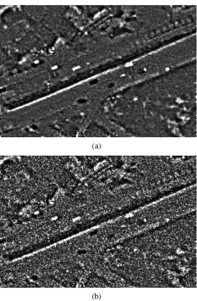
Within the road buffer of Figure 1, the result of TV-L1 texture de-composition is shown in Figure 2 and Figure 3, where the piece-wise smoothly-varying pavement background of Figure 2 is sub-tracted from the aerial road imagery to enhance the sharp edges around vehicles in Figure 3. It should be noted that noise is en-hanced too during the subtraction. Gaussian noise is purposely added to the aerial image to provide insight into how noise influ-ences the TV-L1 texture decomposition. Gaussian white noise of mean 0 and standard deviation 0.01 is added to the top image and Gaussian white noise of mean 0 and standard deviation 0.03 is added to the bottom one, as shown in Figure 4. It can be seen that the homogeneity of the pavement texture becomes a little affect-ed by random noise, which affects the discriminative capability of texture.
3. VEHICLE SHAPE SALIENCY
Figure 1: Road buffer
Figure 2: Pavement background of the cartoon part of the TV-L1 texture decomposition
Figure 3: Enhanced texture around vehicles
3.1 Pavement Surface Detection
Based on the given vector of the road network of the high-resolution aerial image, road extraction is narrowed within the buffer of a certain distance away from the road centerline. However, the road buffer can not exactly cover the whole pavement if the road cen-terline is not accurate and the buffer width is too small. In our algorithm, the buffer width is slightly larger than the number of pixels that total width of all lanes in the aerial image contains. On the one hand, the vehicles will not be missed. On the other hand, using the loose width of road buffer, the extra interferences aris-ing from the roadside buildaris-ings, vegetation, etc. will be excluded in the further procedure. It is a trade off between the accuracy and computational efficiency. The buffer width can be set according to the prior knowledge of the road grade and the spatial resolution of the aerial image.
Instead of extracting vehicles directly, the proposed algorithm s-tarts with the detection of the significant pavement surface. It is based on the fact that pixels being pavement are the majority a-mong those pixels of the road buffer. Also, the central vehicles on the pavement surface are differentiated from the surrounding pavement, because they have quite different intensity and texture from their neighborhood. Meanwhile, road buffer involves not
(a)
(b)
Figure 4: Effects of Gaussian noise.(a)Add Gaussian white noise of mean 0 and standard deviation 0.01. (b)Add Gaussian white noise of mean 0 and standard deviation 0.03.
only pavement but the central and road-side interference afore-mentioned. Pavement surface detection robustly excludes the dis-turbing interference while preserving the outstanding vehicles in the center. This work can be applied in various conditions due to the homogeneity of the pavement texture. It consists of:
1. finding seeds of pavement surface;
2. growing pixels of pavement surface by texture similarity;
3. and morphological closing.
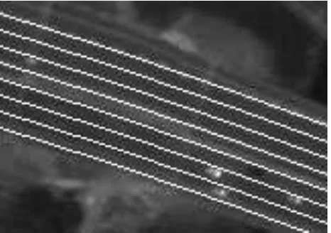
3.1.1 finding seeds of pavement surface Road seeds are lo-cated near the road center and surrounded by pixels that have similar texture. It can be found along the direction perpendicular to the road vector. The number of pixels that satisfy the charac-teristic of seed is comparatively large in the large aerial image. Therefore, every road vector of the road network is sub-sampled every a certain interval during the seed-finding. Seeds are those pixels that have homogenous texture in the neighborhood and a-long the normal direction of the sampled point of the road vector, as shown in Figure 5. Every small buffer area of each road seg-ment has its own seeds, which adapts to the variation of paveseg-ment texture.
Figure 5: Seeds in road buffer. The center of every small circle represents the seed.
begin the search in a breadth-first way. If the difference between the seed and its neighborhood is under the tolerance, the point will be classified as pavement pixel and added to the set of pave-ment surface. At each step, only eight immediate neighbors are considered, and the points having similar texture are picked as new seeds. This process is iterated until it reaches the boundary of the road buffer or the texture difference of neighboring pixel is beyond the threshold. A detailed illustration of the smart routing procedure is given in Figure 6, where numbers inside the grids are texture value. Seed are marked with red color and we assume that the pixel at (3, 4) is the starting seed. Considering the dis-crepancy with its neighborhood, we gather points from (2, 4) to (2, 3) in a clockwise order. It can be seen the pixels collected during the above process are labeled with white color. At each iteration of the loop, one pixel of the pavement surface will be regarded as new starting point, pixels that meet the tolerance of texture difference are added to the queue. Yellow rectangle and green rectangle show the result of the first and second iteration respectively. The process ends up with an empty queue of seeds. Starting with the seeds of Figure 5, the grown pixels of pavement surface are shown in Figure 7.
Figure 6: An overview of the smart routing procedure
3.1.3 morphological closing It can be seen from Figure 7 that most interference from the road-side trees and central iso-lation guardrail is reduced after seed-growing. But there are still many holes and discontinuity in the pavement surface. They are composed of vehicles, lane markings, edges, noise, overlapping bridges, etc. Morphological closing is adopted to eliminate the noise of texture output. The final pavement surface is shown in Figure 8. It should be noted that manual addition of seeds are
Figure 7: Result after growing seeds
readily supported to detect areas of pavement surface that are not well covered by the automatically-chosen seeds. This interactive refinement of the set of seeds enhances the result of pavement surface detection and the accuracy of subsequent vehicle detec-tion.
Figure 8: Result of morphological closing
3.2 Vehicle Shape Saliency
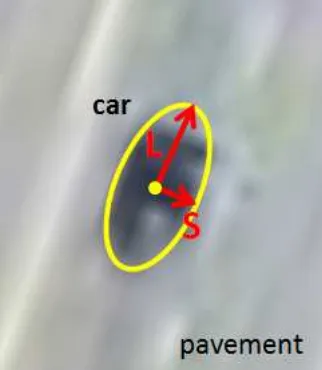
As seen in Figure 9, vehicles are salient holes among the detected pavement surface. Contours of the holes are first analyzed in this section, based on the result of edge drawing in the middle of the road. The vehicle shape saliency is then defined to characterize the rectangular shape saliency of vehicles.
Figure 9: Vehicle shape saliency.Vehicle is marked with yellow border and long and short axis of the ellipse are marked with red.
contour of object is approximated by its principal axis and orien-tation. The approximation is fulfilled by fitting the contour with minimal coverage of ellipse. For every elliptical shapeW, its area, the same as the total pixel numbersNinside the contour, is seen as the sizeaof the vehicle. The rectangular shape saliency
ris given by the ratio of the length of principal axisLand minor axisSof the contour,
L= 2×p2((µxx+µyy) +△) (8)
S= 2×p2((µxx+µyy)− △) (9)
r=L
S (10)
whereµxx,µyy,µxy,△are intermediate variables
µxx=
PN i=1x
2
i
N ;µyy= PN
i=1y 2
i
N ;µxy= PN
i=1xiyi
N (11)
△=p(µxx−µyy)2−4µ2xy (12)
xiandyiare vertical and horizontal coordinates forith coordi-nate of contourW respectively. Based on the physical size and rectangular shape of different vehicle, prior knowledge about the size and rectangular shape saliency can be calculated from the spatial resolution of the aerial image. Contours of bigger or s-maller shape saliency than the prior knowledge will be neglected. Vehicle shape saliency measureS(x)ofxth contour inWis then defined as follows
S(x) =
1 if a∈[10,50], r∈[2,5]
0 else , (13)
where 10, 50 denotes the minimal and maximal area; 2 and 5 represents the probable smallest and largest ratio respectively. All these parameters are dependent on the type of vehicle and the spatial resolution of the aerial image. The measureS(x)indicates 0 and 1 distribution. If the value is 1, it means that the contour is a vehicle. Its centroid represents the occurrence of the vehicle. The contour is discarded when the value is 0. The final result is shown in Figure 13.
3.3 Lane Boundary Localization
As can be seen in Figure 10, the contrast between the vehicle and the road is enhanced by the application of TV-L1 model. Howev-er, the lane boundary is heightened simultaneously. The discrep-ancy of shape saliency between the vehicle located on the top left of Figure 10 and the lane boundary is very small. This will re-sult in the vast erroneous. To differentiate the short lane marking from the vehicle, the lane boundary is located. Vehicles can not be removed because they are always located at the lane center, instead of the lane boundary.
The road centerline contains abundant information about the pave-ment, such as orientation, location, length, etc, and lane bound-aries are parallel with the centerline. The centerline is extracted by the obvious gradient feature and a smart edge detection al-gorithm called Edge Drawing (ED) (Topal and Akinlar, 2012). Based on edges of ED, the next step is fitting the edge pixels in-to the road centerline. According in-to the design specification of road structure, polynomial fitting function is chosen to match the centerline. The width of vehicle lane is a prior knowledge, de-pending on the spatial resolution of aerial imagery. Therefore, lane boundaries can be located easily by translating the center-line curve and under the guidance of the short lane markings on pavement surface. The edge result of ED is shown in Figure 11 and the final result of the lane boundary in Figure 12. The salient
object will be eliminated if its center is located on lane bound-aries. The experimental result demonstrates it can suppress the erroneous effectively.
Figure 10: Interferences of lane boundary.
Figure 11: Result of Edge Drawing. Road centerline and short lane marking are extracted.
Figure 12: Result of lane boundary localization.
4. EXPERIMENTAL RESULTS
image is the GF-2 image of Wuhan, China with a nominal res-olution of 1 m , and provided by China Highway Engineering Consulting Corporation (CHECSC). It can be seen that roads on the right of the image are composed of concrete and surrounded by trees, buildings, etc., while the left is asphalt including many lane boundaries and shadows. Moreover, the colors and the sizes of vehicles vary a lot. This imagery involves different traffic sit-uations and density in a city.
Since we want to get a desired result in such broad and various areas, a loose buffer width of 25 pixels is chosen. This is also why pavement surface detection is applied to refine the buffer. When theλ(a parameter of TV-L1) is set to 1, the detected texture of road is smooth. But a largeλcan also blur the contours of black vehicles. To maintain the black vehicles, the process of TV-L1 is adopted with aλof 0.1. Based on the statistics of vehicles of different types, the shape saliency parameter of area and aspect ratio is set to 10-50 and 2-5 respectively.
To assess the effect of the proposed vehicle detection algorithm, accuracy is the most important. The measureT Pis defined as the geometric ratio based on the number of vehicles and the result of detection as Equation 14 shown. In addition,F Pis calculated as the false alarms as Equation 15 illustrated.
T P = Nt Np
; (14)
F P=Nf
N ; (15)
whereNtrepresents the number of correctly detected vehicles, andNpis the number of vehicles in high-resolution aerial image.
Nf is the number of the contours that are mistakenly detected as vehicles, andNis the total number of output of vehicle detection with our algorithm. Computation time is also recorded to evaluate our proposed algorithm.
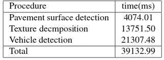
Table 1: Computation time of each procedure.
The computation time is obtained with a PC of an Intel 2.4GHz i7-5500U CPU and 8GB RAM. The total computation time is 39.13 seconds for a4656×3496aerial image. The computation time of each procedure is listed in Table 1. The first procedure takes 4.07s, and includes three steps: constructing the road buffer, growing pavement and morphological closing. The second proce-dure takes 13.75s. This proceproce-dure is texture decomposition using TV-L1 model. The last procedure takes 39.13s and includes two steps: lane boundary localization and vehicle shape saliency de-tection. The 54% of the total computation time is spent on the last procedure. The lane boundary localization can be sped up by an efficient parallel algorithm.
Based on the Equation 14 described ahead,T Pcan be gathered by the difference between our automatic algorithm and visual in-spection. The experimental imagery includes 158 manually col-lected vehicles of which 113 vehicles are correctly detected. Fur-thermore, 31 contours are mistakenly detected as vehicles among the 144 output of the proposed algorithm. Therefore, these results lead to an accuracy of 71.5% and a false alarm of 21.5%.
The result of vehicle detection is shown in Figure 14, with the local vehicle detection results shown in Figure 16-19. Figure 16,
17, and 18 correspond to the region 1, 2, and 3 of Figure 14 re-spectively. Some objects at the lane center could be mistakenly extracted because their shape contours is similar to the vehicle, as shown in Figure 16. In Figure 17(b), a little black vehicles are missed, because they show a very low contrast with their sur-roundings. The missed vehicle is mainly caused by the low con-trast between the vehicle and the road. The vehicles nearby the lane boundary can not be detected in Figure 18. As shown in Figure 18(a), the lane boundary is salient after texture decom-position. Therefore, the vehicle contour is included in the lane boundary contour. These vehicles are missed, because the shape saliency of the lane boundary contour is not satisfied. The Figure 19 shows the good result on concrete pavement. Our algorithm is able to detect vehicles regardless of the colors and the sizes of the vehicle.
Figure 13: Result of vehicle detection. Vehicle detection result is marked by red point.
Figure 14: Result of the proposed algorithm. Three regions are marked with yellow rectangles. Local results of three regions is illustration in Figure 16-18 respectively.
-5. CONCLUSION AND RECOMMENDATIONS
Vehicle detection is important for all transportation agencies to collect the necessary data for optimal allocation of transportation infrastructure. With ever-improving resolution of aerial image, it can contain more precise spatial and spectral information of the vehicles. However, due to the various pavement textural noise, shadow, surface debris, etc, it remains a challenge to detect ve-hicles from the aerial imagery. This paper is motivated to detect vehicles of aerial image in the context of a road and from the shape saliency perspective.
ve-Figure 15: Texture image of whole imagery.
(a) (b)
Figure 16: Illustration of local result.(a)Texture image. (b)Vehicle detection result is marked by red point, object located on lane center is mistakenly detected.
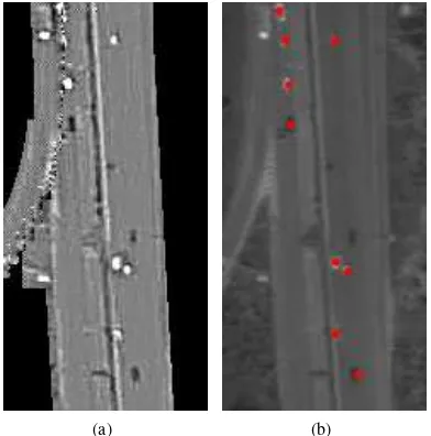
(a) (b)
Figure 17: Illustration of local result.(a)Texture image. (b)Vehicle detection result is marked by red point, several black vehicles are not detected.
hicles using TV-L1 texture decomposition. The interference of different roadside objects is reduced using pavement surface
de-(a) (b)
Figure 18: Illustration of local result.(a)Texture image. (b)Vehicle detection result is marked by red point, vehicles n-earby the road centerline are missed.
(a)
(b)
Figure 19: Illustration of local result.(a)Texture image. (b)Vehicle detection result is marked by red point, vehicles are well detected on concrete pavement.
tection. Based on the TV-L1 texture analysis, the contrast be-tween the vehicles and the road is enhanced. The vehicle shape saliency is chosen to characterize the shape feature of the vehi-cles, which opens the door to detect vehicle of different size and color. To suppress the erroneous effectively, the lane boundary is localized by centerline drawing and displacement. The proposed algorithm is tested on an aerial image with the size of4656×3496
pixels that contains complicated road structure, different setting surrounding the roadside, different sizes and colors of vehicles, etc. Experimental results show the proposed algorithm can detect vehicles with various sizes and colors in different pavement tex-ture. It is promising for the automatic classification of vehicles of different types from the aerial imagery.
Although the proposed algorithm demonstrates its capability for vehicle detection, we recommend that:
1. more comprehensive tests be conducted for various aerial data, including a diverse set of Very High Resolution (VHR) images of different traffic density.
3. other vehicle salient features, such as color, orientation, shape, etc. be combined with the proposed vehicle shape saliency measure.
ACKNOWLEDGEMENTS
The authors are grateful for the support of the demonstrative trans-portation research and development program using GF-2 high-resolution aerial imagery, P.R.China ( NO: 07-Y30B10-9001-14/16 ). The authors also give many thanks to Tian Zhou and Jian Wang for their great work on the prototype development of this work.
REFERENCES
Chang, W. C. and Cho, C. W., 2010. Online boosting for vehicle detection. IEEE Transactions on Systems, Man, and Cybernetics, Part B (Cybernetics) 40(3), pp. 892–902.
Cheng, H. Y., Weng, C. C. and Chen, Y. Y., 2012. Vehicle de-tection in aerial surveillance using dynamic bayesian networks. IEEE Transactions on Image Processing 21(4), pp. 2152–2159.
Elangovan Vinayak, A. B. and Amir, S., 2013. A multi-attribute based methodology for vehicle detection and identification. Proc. SPIE 8745, pp. 87451E–87451E–10.
Gavrila, D. M.and Munder, S., 2006. Multi-cue pedestrian detec-tion and tracking from a moving vehicle. Internadetec-tional Journal of Computer Vision 73(1), pp. 41–59.
Hsieh, J.-W., Chen, L.-C. and Chen, D.-Y., 2014. Symmetrical surf and its applications to vehicle detection and vehicle make and model recognition. IEEE Transactions on Intelligent Trans-portation Systems 15(1), pp. 6–20.
Le Guen, V., 2014. Cartoon+ texture image decomposition by the tv-l1 model. Image Processing On Line 4, pp. 204–219.
Leitloff, J., Hinz, S. and Stilla, U., 2010. Vehicle detection in very high resolution satellite images of city areas. IEEE Transactions on Geoscience and Remote Sensing 48(7), pp. 2795–2806.
Mithun, N. C., Rashid, N. U. and Rahman, S. M. M., 2012. De-tection and classification of vehicles from video using multiple time-spatial images. IEEE Transactions on Intelligent Trans-portation Systems 13(3), pp. 1215–1225.
Sivaraman, S. and Trivedi, M. M., 2011. Active learning for on-road vehicle detection: a comparative study. Machine Vision and Applications 25(3), pp. 599–611.
Stefan, H., Dominik, L. and Jens, L., 2008. Traffic extraction and characterisation from optical remote sensing data. The Pho-togrammetric Record 23(124), pp. 424–440.
Sun, Z., Bebis, G. and Miller, R., 2002. On-road vehicle detection using gabor filters and support vector machines. Digital Signal Processing, 2002. DSP 2002. 2002 14th International Conference on 2, pp. 1019–1022 vol.2.
Topal, C. and Akinlar, C., 2012. Edge drawing: a combined real-time edge and segment detector. Journal of Visual Communica-tion and Image RepresentaCommunica-tion 23(6), pp. 862–872.
Zheng H, Pan L, L. L., 2006. A morphological neural network approach for vehicle detection from high resolution satellite im-agery. Neural Information Processing - 13th International Con-ference 4233 LNCS - II, pp. 99–106.