EXPLICITLY ACCOUNTING FOR UNCERTAINTY IN CROWDSOURCED DATA FOR
SPECIES DISTRIBUTION MODELLING
D. Rocchinia∗, A. Comberb, C.X. Garzon-Lopeza, M. Netelera, A.M. Barbosac, M. Marcantonioa, Q. Groomd, C. da Costa Fontee, G.M. Foodyf
aDepartment of Biodiversity and Molecular Ecology,
Research and Innovation Centre,
Fondazione Edmund Mach, Via E. Mach 1, 38010 S Michele allAdige, TN, Italy bThe School of Geography, University of Leeds Leeds, LS2 9JT, UK c
Centro de Investigacao em Biodiversidade e Recursos Geneticos (CIBIO), InBIO Research Network in Biodiversity and Evolutionary Biology,
University of Evora, 7004-516 Evora, Portugal d
Information Technology and Botany - Botanic Garden Meise, Brussels, Belgium e
Universidade de Coimbra, Portugal f
School of Geography, University of Nottingham, University Park, Nottingham NG7 2RD, UK
Commission II, WG II/4
KEY WORDS:Ecosystems, Fuzzy Sets, Sampling Bias, Sampling Effort, Semantic Problems in Species Determination, Species Distribution Models, Uncertainty
ABSTRACT:
Species distribution models represent an important approach to map the spread of plant and animal species over space (and time). As all the statistical modelling techniques related to data from the field, they are prone to uncertainty. In this study we explicitly dealt with uncertainty deriving from field data sampling; in particular we propose i) methods to map sampling effort bias and ii) methods to map semantic bias.
1. INTRODUCTION
In ecology, a number of studies have dealt with the prediction of species distribution and diversity over space and its changes over time based on a set of environmental predictors related to envi-ronmental variability, productivity, spatial constraints and climate drivers.
Species distribution models have been acknowledged as the most powerful methods to map the spread of plant and animal species. The basic approach used to create maps based on predictors is to rely on linear models to create gridded landscapes of potential distribution of species based on point or polygon local data.
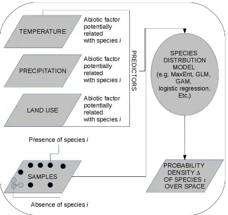
In most cases, the output is a density function in two dimen-sions representing the distributionSx of thexspecies. In gen-eral boundaries are sharply defined based on thresholds of pre-dictors/factors (e.g. when mainly based on land cover, see also (Comber et al., 2013)) or continuous, if based on the continuous variability of predictors (e.g. the continuous variability of tem-perature). Figure 1 represents an example.
Uncertainty in such models mainly derives from input data pseu-doabsences (Foody, 2011) as well as from models’ bias, i.e. the error deriving from the model being chosen (GAM, GLM, Maxi-mum entropy models, etc,).
Hence, the representation of uncertainty in two dimensions is strongly suggested although it is disregarded in most cases. How-ever, its importance is apparent (Comber et al., 2012). In fact areas with a high or low probability of distribution of a species might be also in relation with a high or low error rate.
∗[email protected], [email protected]
Figure 1: An example of the flow leading to a species distribu-tion map, derived as a probability density funcdistribu-tion from spatial gridded predictors, mainly in raster but also in vector format, and point data in the field.
relation with the following equation:
Decision=
< Em|> I < Em|< I > Em|> I > Em|< I
(1)
In this case a high (or low) invasion rateImight be related to high or low errorEmin the output model being observed by decision makers. The most dangerous situation is achieved when a low predicted invasion rate is related to a high error in the modelling procedure (bottom right part of Eq.(1)). For instance, decision makers might underestimate the effort to be put against invasion rate, suspected to be low from the species distribution map.
Strictly speaking, a misconceived use of a species distribution map might be dangerous e.g. in case of a low probability of dis-persion of an invasive species but with a high error in the model. The prediction of the distribution of an invasive species might be low but with a high error; hence its spread could be underesti-mated in some parts of an area.
The aim of this study is to provide straightforward and robust mapping procedures to explicitly show spatial uncertainty related to sampling problems like sampling effort or crowdsourced se-mantic uncertainty (relying on commonly used datasets) when dealing with species distribution modelling.
2. UNCERTAINTY RELATED TO SAMPLING EFFORT: REPRESENTATION OF SAMPLING BIAS BY TREATMENT OF DIFFUSION AND DENSITY
ALGORITHMS
Concerning bias related to sampling effort, we will rely on one of the mostly used datasets in biodiversity study at large spatial extents, namely the GBIF dataset.
GBIF data comprises a huge range of species occurrence obser-vations collected with a wide variety of sampling approaches, in-cluding observations coming from specimens in museums and herbaria, which are not necessarily systematically collected. It spans from well established plot censuses to direct observations collected during field trips. Consequently, some of the data points are at the center of censused grids (each point comprises the species located at a specific-size quadrant) or correspond to sin-gle observations of one (or more) individuals of the same species. These differences also depend on the methodologies used to ob-serve/record occurrences per taxon. Plots, and plots within sects, are common practice in vegetation censuses, while tran-sects, point counts and live traps are preferred in the case of ani-mals.
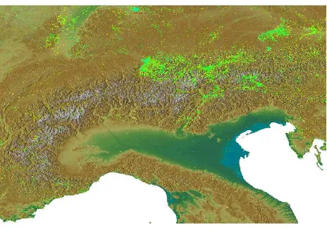
Moreover, the variation in factors such as per country biodiversity monitoring schemes (Figure 2), funding schemes, focal ecosys-tems, accessibility to remote areas (Figure 3), among others, add another source of variation, especially at multinational scales (Bar-bosa et al., 2013).
Undoubtedly, all those sources of variation result in a non ho-mogeneous sampling that has important consequences not only on the development of accurate species distribution maps but, more importantly, on the conservation and management decisions focused on such a distribution of biodiversity (Rocchini et al., 2011). The aim of this study was to explicitly show spatial un-certainty in the sampling effort of the GBIF data, by explicitly taking into account potential area effects of European countries.
Figure 2: Plants occurrences for Europe per country extracted from GBIF data (website accessed Dec 2014). The areas in white have zero occurrences recorded in the GBIF database. A higher sampling density is represented moving from green to blue colour. This figure was developed by GRASS GIS software (Neteler et al., 2012).
Figure 3: Plant occurrences and topography in the Alps region (Europe). Plant occurrences extracted from GBIF data (web-site accessed Dec 2014). Light green points (observations from GBIF) follow valleys within Alps, i.e. the most accessible points. This Figure was developed by GRASS GIS software (Neteler et al., 2012). Refer to the main text for additional information.
In this study we aim at quantifying and mapping the uncertainty derived from the variation in observations due to differences in sampling efforts (Figures 2, 3). In particular the use of cartograms is proposed, in which the shape of objects (countries) is directly related to a certain property, in our case to uncertainty. Car-tograms build on the standard treatment of diffusion, in which the current density is given by:
J=v(r, t)p(r, t) (2)
where v(r, t) and p(r, t) are the velocity and density at position r and time t. Refer to (Gastner and Newman, 2004) for additional information.
den-sity of information contained (number of observations, variation, etc). For example, using this strategy the generated maps show the differences in species observations per country in all taxa and in some of the main taxa (Figure 4).
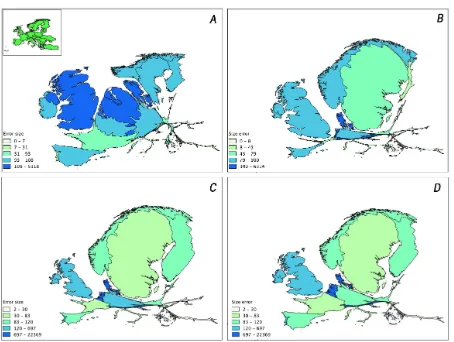
The cartograms were developed using the free and open source software ScapeToad (http://scapetoad.choros.ch/). The shape and final area of the countries will derive from the difference between the actual size of the country and the size of the sampling (e.g., the number of observations). Hence, smaller areas which are comparatively oversampled will look bigger in the cartograms, with a higher sampling density, while bigger comparatively over-sampled areas will have a high value but a lower relative size. Hence the method directly accounts for the area effect, i.e. the size of each country, on the final sampling effort. As an example, in Figure 4 the Netherlands and Sweden show a higher sampling density (see the Southern part of Sweden of Figure 2), but the lat-ter occupies a bigger surface. Hence in the final cartogram (e.g. Figure 4A), the higher sampling density of the Netherlands is en-hanced by both values (colour) and shape (final occupied areas).
In the proposed method, uncertainty is shown at the per country scale and corresponds to the deformation of the original coun-try area, that is, countries smaller than their original size require more sampling effort concerning the products derived from the GBIF data.
Figure 4: Cartogram of species occurrences. Extracted from GBIF data (website accessed December 2014). Error size above 100 indicates higher sampling density and error size below 100 indicates the country in under-sampled. A) Plants; B) Fungi; C) Animals; D) All taxa.
The method can be applied also taking into account the tempo-ral scale. An example is provided considering plant species data (Figure 5). In this case, undersampling in the southern part of Eu-rope is clear considering three different periods (Figure 5A) and the final cumulated data (Figure 5B). As previously stated, this is not actually related just to field sampling but mainly to data sharing. Since sampling effort bias might affect final results in species distribution modelling, future developments will include the visualization of species distribution model predictions com-bined with the map of uncertainty presented here.
Figure 5: Cartogram of plant species occurrences at different dates, considering different periods (A) and cumulated data (B). Extracted from GBIF data (website accessed December 2014).
3. SEMANTIC UNCERTAINTY: POTENTIAL OF FUZZY SET THEORY TO MODEL CROWDSOURCED DATA UNCERTAINTY
Beside sampling bias, shown in the previous section, taxonomic bias, related to thematic (semantic) accuracy, might occur when different operators / scientists deal with the association of each individual to a certain species / class / taxon.
There are a number of provoking papers dealing with problems in the discrimination of species in the field, including operator bias (Bacaro et al., 2009), taxonomic inflation (Knapp et al., 2005) and more generally taxonomic uncertainty (Guilhaumon et al., 2008), i.e., the subjectivity of field biologists in acquiring species lists which is expected to increase error variance instead of obtaining accurate information on field data.
Fuzzy set theory should aid in maintaining uncertainty informa-tion related to each species (hereafter also generally related to class as in fuzzy set theory). The concept of fuzzy sets was first introduced by (Zadeh, 1965); thus, fuzzy set based approaches have been widely used in ecology dating back to 1980s (see (Comber et al., 2012)).
The principle behind fuzzy set theory is that the situation of one class being exactly right and all other classes being equally and exactly wrong often does not exist. Conversely, there is a gradual change from membership to non-membership (Gopal and Wood-cock, 1994).
Fuzzy sets have been used in a number of fields where abrupt thresholds (classes) cannot represent a suitable model of reality, including: massive data analysis and computation (Jasiewicz and Metz, 2011), expert knowledge (Janssen et al., 2010-05-10), the-oretical topological spaces (Ghareeb, 2011-04), species habitat suitability modeling (Amici et al., 2010), soil science (Burrough et al., 1997), and vegetation science (Foody, 1996).
A fuzzy set is defined as follows: let U denote a universe of enti-ties u, the fuzzy set F turns out to be:
F = (u, µ(u))|u∈U (3)
where the membership function associates for each entity u the degree of membership into the set F.
The degree of membershipµ(u)ranges in the interval [0,1], i.e. the real range between 0 and 1.
Hence, fuzzy sets might represent a good starting point for con-tinuously mapping species, by relying on each species as:
F j= (u, µj(u))|u∈U (5)
In this case, for each speciesiandja map is derived based on e.g. fuzzy training data taken in the field (probability of each individ-ual to belong to a certain species) representing species probabil-ity of occurrence. In this case, according to (Boggs, 1949) un-certainty is explicit in the sense that a probability of occurrence of each sampled individual to each species is mapped instead of a crisp set considering that species as exhaustively determined, with a 100% accuracy.
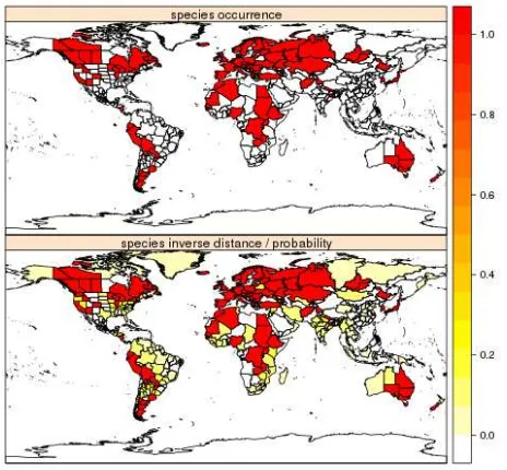
One major assumption leads to consider fuzzy sets as a pow-erful tool for maintaining uncertainty information when aiming at mapping and analysing species or in general taxa distribution patterns, i.e. the gradual and continuous probability of correct determination of a certain species rather than considering a com-plete accuracy in the determination process. A fuzzy determina-tion of a species might be derived as an example as the probabil-ity of correct determination given different operators / scientists. Figure 6 represents an example for the foraminifera species Ker-atella quadrata. A map of presence of the species worldwide (per country / region) is shown together with the probability (as in-verse distance) of occurrence of each individual with the species / group. The analysis was performed relying on thefuzzySym package (Barbosa, 2015) for the R software. One of the assump-tions of the package and the related paper (Barbosa, 2015) is that an individual does not “belong” to a certain species, but it has a probability of inclusion in that species based on human-based classification / determination. From a theoretical point of view this is similar to approximation theory in mathematics, in which, once searching for a function which best approximates a more complex one, the characterization of the introduced errors (un-certainty) is of primary importance (e.g., (Fourier, 1822)).
Figure 6: Representation of the presence of the foraminifera speciesKeratella quadrata and the probability (as inverse dis-tance) of occurrence of each determined individual to that species. While the presence / absence map has obviously only red (1 - presence) and white (0 - absence) colour, the probability map based on inverse distance covers the whole range of decimal values from 0 to 1.
4. CONCLUDING REMARKS
The description of local and global uncertainty variation over space of species distribution models is mandatory since SDMs are the main practical tool for decision makers to manage and conserve biodiversity. Determining and mapping uncertainty can help users to assess the suitability of such models, for which geo-graphical analysis is fundamentally concerned with how and why processes vary spatially (Comber, 2013).
Because of spatial nonstationarity, the parameters of the model describing the distribution of a species and the related uncertainty may vary greatly in space, limiting the descriptive and predictive utility of global models (Foody, 2004).
Ecologists and landscape managers and planners must seriously take into account uncertainty in both input data sampling effort and semantics to deal with reliable species distribution maps. As previously stated (see Eq.(1)), if such uncertainty is not taken into account, final decisions on species conservation might be biased by input errors.
In this study we dealt with spatial uncertainty in species distribu-tion modelling deriving from two main issues related to field data sampling: sampling bias and semantic issues. The approaches proposed in this study to explicitly map spatial uncertainty are based on free and open source software. We argue that they might represent straightforward, robust and reproducible methods to ex-plicitly account for uncertainty when dealing with species distri-bution modelling.
ACKNOWLEDGEMENTS
This study has been funded by the COST Action TD1202 ”Map-ping and the Citizen Sensor” funded by the European Union. Duccio Rocchini and Carol X. Garzon-Lopez are partially funded by the EU BON (Building the European Biodiversity Observation Network) project, funded by the European Union under the 7th Framework programme, Contract No. 308454. Duccio Rocchini is also partially funded by the ERA-Net BiodivERsA, with the national funders ANR, BelSPO and DFG.
REFERENCES
Amici, V., Geri, F. and Battisti, C., 2010. An integrated method to create habitat suitability models for fragmented landscapes. Jour-nal for Nature Conservation 18(3), pp. 215–223.
Bacaro, G., Baragatti, E. and Chiarucci, A., 2009. Using taxo-nomic data to assess and monitor biodiversity: are the tribes still fighting? 11(4), pp. 798–801.
Barbosa, A., 2015. fuzzySim: applying fuzzy logic to binary similarity indices in ecology. Methods in Ecology and Evolution p. in press.
Barbosa, A. M., Pautasso, M. and Figueiredo, D., 2013. Species-people correlations and the need to account for survey effort in biodiversity analyses. Diversity and Distributions 19(9), pp. 1188–1197.
Boggs, S., 1949. An atlas of ignorance: A needed stimulus to honest thinking and hard work. Proceedings of the American Philosophical Society 93(3), pp. 253–258.
Comber, A., 2013. Geographically weighted methods for esti-mating local surfaces of overall, user and producer accuracies. Remote Sensing Letters 4(4), pp. 373–380.
Comber, A., Fisher, P., Brunsdon, C. and Khmag, A., 2012. Spa-tial analysis of remote sensing image classification accuracy. Re-mote Sensing of Environment 127, pp. 237–246.
Comber, A., See, L., Fritz, S., Van der Velde, M., Perger, C. and Foody, G., 2013. Using control data to determine the reliability of volunteered geographic information about land cover. Interna-tional Journal of Applied Earth Observation and Geoinformation 23, pp. 37–48.
Foody, G., 1996. Fuzzy modelling of vegetation from remotely sensed imagery. Ecological Modelling 85(1), pp. 3–12.
Foody, G. M., 2004. Spatial nonstationarity and scale-dependency in the relationship between species richness and en-vironmental determinants for the sub-saharan endemic avifauna. Global Ecology and Biogeography 13(4), pp. 315–320.
Foody, G. M., 2011. Impacts of imperfect reference data on the apparent accuracy of species presence?absence models and their predictions. Global Ecology and Biogeography 20(3), pp. 498– 508.
Fourier, J., 1822. Thorie Analytique de la Chaleur. Didot, Paris.
Gastner, M. and Newman, M., 2004. Diffusion-based method for producing density-equalizing maps. Proceedings of the National Academy of Sciences USA.
Ghareeb, A., 2011-04. Normality of double fuzzy topological spaces. Applied Mathematics Letters 24(4), pp. 533–540.
Gopal, S. and Woodcock, C., 1994. Theory and methods for accu-racy assessment of thematic maps using fuzzy sets. Photogram-metric Engineering and Remote Sensing 60(2), pp. 181–188.
Guilhaumon, F., Gimenez, O., Gaston, K. and Mouillot, D., 2008. Taxonomic and regional uncertainty in species-area relationships and the identification of richness hotspots. Proceedings of the National Academy of Sciences of the United States of America 105(40), pp. 15458–15463.
Janssen, J., Krol, M., Schielen, R., Hoekstra, A. and de Kok, J.-L., 2010-05-10. Assessment of uncertainties in expert knowl-edge, illustrated in fuzzy rule-based models. Ecological Mod-elling 221(9), pp. 1245–1251.
Jasiewicz, J. and Metz, M., 2011. A new grass gis toolkit for hor-tonian analysis of drainage networks. Computers & Geosciences 37(8), pp. 1162–1173.
Knapp, S., Lughadha, E. and Paton, A., 2005. Taxonomic infla-tion, species concepts and global species lists. 20(1), pp. 7–8.
Neteler, M., Bowman, M. H., Landa, M. and Metz, M., 2012. Grass gis: A multi-purpose open source gis. Environmental Mod-elling & Software 31, pp. 124–130.
Rocchini, D., Hortal, J., Lengyel, S., Lobo, J., Jimnez-Valverde, A., Ricotta, C., Bacaro, G. and Chiarucci, A., 2011. Account-ing for uncertainty when mappAccount-ing species distributions: the need for maps of ignorance. Progress in Physical Geography 35(2), pp. 211–226.