AD HOC MODEL GENERATION USING MULTISCALE LIDAR DATA FROM A
GEOSPATIAL DATABASE
M. Gordon∗, B. Borgmann, J. Gehrung, M. Hebel, M. Arens
Fraunhofer Institute of Optronics, System Technologies and Image Exploitation IOSB Ettlingen, Germany
[email protected], [email protected], [email protected], [email protected], [email protected]
http://www.iosb.fraunhofer.de
Commission III, WG III/5
KEY WORDS:LIDAR, Database, Model, Mapping, Visualization, Urban
ABSTRACT:
Due to the spread of economically priced laser scanning technology nowadays, especially in the field of topographic surveying and mapping, ever-growing amounts of data need to be handled. Depending on the requirements of the specific application, airborne, mobile or terrestrial laser scanners are commonly used. Since visualizing this flood of data is not feasible with classical approaches like raw point cloud rendering, real time decision making requires sophisticated solutions. In addition, the efficient storage and recovery of 3D measurements is a challenging task. Therefore we propose an approach for the intelligent storage of 3D point clouds using a spatial database. For a given region of interest, the database is queried for the data available. All resulting point clouds are fused in a model generation process, utilizing the fact that low density airborne measurements could be used to supplement higher density mobile or terrestrial laser scans. The octree based modeling approach divides and subdivides the world into cells of varying size and fits one plane per cell, once a specified amount of points is present. The resulting model exceeds the completeness and precision of every single data source and enables for real time visualization. This is especially supported by data compression ratios of about90%.
1. INTRODUCTION
Due to the rapid technological development in recent years, 3D sensors have found a high degree of dissemination in research and development. Thus today airborne, mobile or terrestrial laser scans are collectable with much less effort than a decade ago, which makes them an easily available data source for topographic surveying and mapping. As each sensor system has a distinct res-olution, accuracy and precision and due to the available flood of data, real time visualization and decision making based on naive point cloud rendering is not feasible. Current state of the art workstations are seldom able to visualize larger terrains due to the sheer mass of millions and billions of points, even if they utilize multiple graphic cards. In addition to the visualization problem, the efficient storage and easy recovery, so that for example one is able to select data based on regions of interest (ROI) or other spatial parameters, is a challenging task.
As an approach to solve this problem, we propose a method for the intelligent storage of 3D point clouds in a geodatabase. Along with the data set, its geolocation and additional meta information are stored. Because a given ROI is typically a geographically bounded area, our approach is able to extract the related data from the database. Additional meta information based search pa-rameters like date or time enable further query refinement. All returned point clouds are fused in a model creation process. Due to the fact that many points could be represented by a common surface, they could be considered as redundant. As most parts of an urban environment are flat, we’ve chosen a plane as mostly ex-pressive representation for a given subset of points. In combina-tion with this plane-based representacombina-tion, an octree data structure is used to handle the huge amounts of data. This approach was
∗Corresponding author.
first presented in (Gordon et al., 2015) and is adapted to incorpo-rate data sources with different accuracy and precision.
2. RELATED WORK 2.1 Spatial data storage
Working with large quantities of georeferenced spatial data re-quires efficient management techniques. While classical data-bases permit searching for information in an efficient way, search requests based on spatial parameters like regions or the distance to a given point assume specialized capabilities on the database side. Aspatial databaseprovides special data types for geometric objects which allow it to store geographic data in regular database tables. It also provides functions and indexes to query and ma-nipulate the data using some kind of SQL like language (Obe and Hsu, 2011). This not only ensures the spatial deposition, but also enables the analysis of the stored data in terms of complex queries like ”give me all point clouds ordered by accuracy that are within range of a camera track that crossed a given region.”
Despite the fact that spatial data storage is a relatively new chap-ter in the history of databases, a variety of implementations ex-ists. The following section is focused on a quick overview of the most common open source solutions. In terms of non-relational database management systems (DBMS), various solutions like MongoDB, BigTable, Cassandra and CouchDB provide spatial support. On the relational side, a lightweight spatial DBMS based on SQLite isSpatiaLite1. It requires no complex client-server ar-chitecture and stores the database in a local file. The popular SQL based DBMSMySQL2provides a spatial extension since version
1
https://www.gaia-gis.it/fossil/libspatialite/index
2
4.1, as stated in the official documentation. It is based on the ”OpenGIS
R
Implementation Standard for Geographic informa-tion - Simple feature access - Part 2: SQL opinforma-tion” of the Open Geospatial Consortium. Unfortunately not all features stated in the white paper seem to be implemented. PostGIS3is an exten-sion of the PostgreSQL4 object-relational DBMS. It is consid-ered to be the open source spatial DBMS with the largest range of functions and also seems to be widely used, among others by the OpenStreetMap project.
2.2 Surface Reconstruction
The surface reconstruction from point clouds is a long standing problem with different solutions. An overview is given e.g. in (Remondino, 2003). A related problem is the (iso)surface extrac-tion from volumetric data (for example generated by computer tomographs). One class of surface reconstruction algorithms gen-erates a mesh to connect the points of the point cloud (e.g. (Mar-ton et al., 2009)). Another way is to generate an implicit function and to use a surface extraction method afterwards, like march-ing cubes (Lorensen and Cline, 1987). A similar approach is de-scribed in (Hoppe et al., 1992).
A different solution is the grouping of points, which have some-thing in common, like forming a geometric primitive (e.g. plane or sphere), cf. (Vosselman et al., 2004). A region growing ap-proach for plane extraction and a subsequent convex hull deter-mination for polygon generation is presented in (Vaskevicius et al., 2007). To speed up the plane extraction, the methods in the following publications separate the points into cells, either grid or octree, and try to extract a plane per cell: A grid approach with RANSAC plane extraction is shown in (Hansen et al., 2006). Two similar solutions using an octree data structure are presented in (Wang and Tseng, 2004) and (Jo et al., 2013). Both try to ex-tract a plane in one cell and divide it, until a sufficient solution is found. In (Wang and Tseng, 2004) least square plane fitting is used, followed by a merge-strategy during postprocessing. (Jo et al., 2013) exploit the regular pattern of the TOF camera for “microplane” estimation and check if all “microplanes” in a cell match, given an error bound.
2.3 Contribution
Our basic idea is to combine a geospatial database with an exist-ing model creation approach. The database provides a scaleable and automatic way to handle the georeferenced data and it has the ability for easy and fast data selection. To use the supplied data in the model generation, the existing approach (Gordon et al., 2015) had to be extended. Therefore a data fusion concept is pre-sented, which is based on the standard deviation of the different data sources. The standard deviation of the point positioning ac-curacy is used for the threshold calculation of the point-to-plane distance and is also applied as a weighting factor for the principal component analysis. In this way, 3D data from different sources can easily be combined.
3. METHOD
Regarding the data used by our approach we assume that it is al-ready georeferenced and stored in a database. The procedure pre-sented here consists of two parts: At first all data sets with a max-imal range from a given position are queried from the database. Then the resulting point clouds are handed over to the model cre-ation process.
3
http://postgis.net
4
http://www.postgresql.org
We continue with an introduction of ourGeo Database. After-wards we give a comprehensive description of the model creation. The section concludes with a parameter overview and implemen-tation details.
3.1 Data handling with Geo DB
For georegistered storage, management and easy retrieval of bi-nary data, such as sensor measurements, we have developed a geospatial database. This database contains meta information to describe the binary data. This allows it to fast retrieve sensor data based on these meta information, which is used as part of our approach.
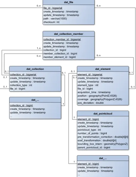
Figure 1 shows an entity-relationship (ER) diagram of that part of our database which is relevant to describe our approach. The database is organized in elements and collections. Elements are the smallest units of information. They could be organized in collections for example to combine all data of one measuring campaign. There are several specialized types of elements and collections which are used to fulfill the special requirements with regard to the meta information we want to store for different types of data. We store point clouds as a specialized version of an ele-ment. This means that, for each point cloud, we have one data set in the ”element” and one in the ”pointcloud” table.
3.2 Model creation
The input to the model creation consists of the point clouds que-ried from the database. They are transformed into a common co-ordinate system and sorted according to the standard deviation in ascending order. The latter allows to start with the most detailed data set and incrementally add the less precise ones. Because the points of different precision are later brought together in a sin-gle representation, each one has to contain the standard deviation associated with the sensor it originates from. Neither the size of the scene nor the number of points need to be known. This is achieved by using a dynamically growing data structure in com-bination with an incremental method. The result is a polygon model, which represents all input points lying on planar surfaces. For visualization and other purposes, also points not represented by the model are preserved. They emerge if their representation by a plane is not possible (e.g. in the case of vegetation) or their neighborhood is too sparse.
The employed data structure is an octree, which can be increased dynamically, if required. Its cell size has a lower bound, which is e.g. defined in accordance with the most precise input source. It also permits a computationally cheap plane extraction. For every cell of the octree, the goal is to have either none or exactly one plane as a representative. The plane fitting is carried out by using a RANSAC (cf. (Fischler and Bolles, 1981)) approach. If mainly outliers are found, that cell is further divided in eight subcells until a certain level of detail is reached (the minimal octree cell size). In case a representing plane can be determined, the data points should additionally be uniformly distributed among this plane. This test is done at the end of the model creation, after all points were added.
We want to combine data of different precision and accuracy. Therefore the value of the standard deviation is incorporated in the generation of a threshold for the point-to-plane distance. In-spired by the fact that68%of normal distributed measurements lie in an interval around the mean bound by the standard devia-tion, the allowed point-to-plane distance is determined by mul-tiplying the standard deviation with a commonsample coverage factor. This allows the combination of points with varying pre-cision. Additionally1/σ2
is used as a weighting factor for the principal component analysis (cf. 3.2.2).
The polygon model itself is created by computing the intersection of each cubical octree cell with the plane assigned to it. This step can be done at any time during the model generation. In the next subsection the details of the point handling are described. Next to that the test of uniform distribution is explained.
3.2.1 Point handling The model creation handles all points sequentially. Assuming that a plane was already fitted to an octree cell, then all points in this cell are divided in a RANSAC manner into support (S) and contradiction set (C). If a new point is added to this cell, its destination set is determined based on the point-to-plane distance. In case of too many outliers, a new plane fit is carried out or finally, if there are still too many outliers, the octree cell is divided.
In case of a previously empty cell or a cell without plane (w.p.), the new point is added to a single set until enough points are collected in this cell. Then a plane fit is performed, and if it suc-ceeded, the two sets (support and contradiction) are determined. Otherwise more points are collected in this cell and the plane fit-ting is retried. However, if a certain number of points is reached without successful plane fitting, the octree cell is divided. The threshold for the plane fitting is based on the point density w.r.t. the squared cell side length and a minimal required number of
points. The details are given as pseudo-code in Algorithm 1, where point density is abbreviated withpd.
Algorithm 1Point handling 1: procedurePOINTHANDLING(p)
2: determine octree cell c of p (create, if not existing) 3: ifc has planethen
4: ifp supports planethen 5: add p to support set (S) of c
6: else
7: add p to contradiction set (C) of c 8: if#C > q∗#Sthen
26: determine S and C
27: end if
28: end if 29: end if 30: end procedure
3.2.2 Test for point-plane coverage This section describes the method that we use to test whether or not the points in a given octree cell are uniformly distributed among the plane assigned to it. The reason to perform this test is to guarantee that the re-sulting planar patch will be a best possible representative of the points it is supposed to replace afterwards. If this constraint is violated, then the cell is further divided into eight subcells. As a positive side-effect, a better estimation of the plane parameters is obtained.
The analysis of the point distribution is carried out using the prin-cipal component analysis (e.g. (Hoppe et al., 1992)). It is only applied to the support set. Assuming that these points lie on a plane, then the two larger eigenvalues (λ1andλ2) represent the
variance of the point distribution along the two major axes of the plane. The square root of the eigenvalues yields the correspond-ing standard deviation.
In case of a one-dimensional uniform distribution, the standard deviation in the interval [a, b]is (b−a)
(2√3). Applied to our problem and under the assumption of nearly uniformly dis-tributed points, l
(2√3) ≈0.28·l(wherelstands for the cell side length) is an upper bound for the square root of the two big-ger eigenvalues. To allow some variation, a smaller threshold is used as a test criterion (√λ1> tand
√
λ2> t). This thresholdt
is calledminimal variation.
sample coverage factor f ∗σ is the maximal allowed point-to-plane distance for both: the point handling and the RANSAC plane fitting.
proportion of outliers Maximal allowed proportion of outliers for both the point handling (cf. qin Algorithm 1) and the RANSAC plane fitting.
RANSAC iterations Number of RANSAC iterations during the plane fitting.
minimal cell size The minimal octree cell size.
dstart Minimal point density needed in a cell before starting plane
fitting (cf.din Algorithm 1).
dmax Upper bound ford(cf.dmaxin Algorithm 1).
kmin Minimal number of points needed for plane fitting (cf.kmin in Algorithm 1).
kmax Upper threshold for number of points, where plane fitting starts independently of point density (cf. kmax in Algo-rithm 1).
minimal variation This valuetis the criterion for uniform dis-tribution of points (see section 3.2.2 for details) .
3.3 Implementation details
All parts of our implementation take advantage of the freely avail-ablePoint Cloud Library (PCL)5(Rusu and Cousins, 2011). Es-pecially its octree implementation was used and extended where needed. The PCL itself uses theVisualization Toolkit (VTK)6for visualization purposes. We additionally utilize the VTK to calcu-late the intersection between an octree cell and a plane in order to get the resulting polygon. For the database we use PostgreSQL and its PostGIS extension.
4. EXPERIMENTS 4.1 Test site
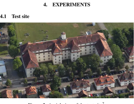
Figure 2. Aerial view of the test site7.
The data acquisition took place in the urban area around the Fraunhofer IOSB in Ettlingen, partly shown in Figure 2. The site containing the institute building, supporting structures and trees is located within a suburban neighborhood. The path driven by the sensor vehicle MODISSA is shown in Figure 3, along with the locations of the terrestrial scan locations.
5
http://pointclouds.org/
6
http://vtk.org/
7
Ettlingen, Fraunhofer Institut IOSB by Wolkenkratzer http://commons.wikimedia.org/wiki/File:Ettlingen, _Fraunhofer_Institut_IOSB.JPG licensed under http: //creativecommons.org/licenses/by-sa/3.0
Figure 3. Path driven by the sensor vehicle (MLS data) during the data acquisition and 23 positions of TLS scanner (Image data: Google Earth, Image c2015 GeoBasis-DE/BKG).
4.2 Experimental setup
The paper describes the fusion of 3D laser scans of distinct ac-curacy with the purpose of generating a model with maximum terrain coverage and precision. To examine the model generation algorithm, multiple data sets were chosen that describe the same urban terrain, but have been recorded from distinct viewing an-gles and using multiple LIDAR systems with different accuracy. Laser scans from airborne, mobile and terrestrial laser scans were utilized. This section gives a short description of all three sensor systems used to record the data.
ALS Airborne laser scanning methods usually combine a time-of-flight LIDAR device with high-precision navigational sensors mounted on a common sensor platform. The deployed Applanix POS AV 410 navigation system comprises a GNSS receiver and a gyro-based inertial measurement unit that measures pitch, roll, and heading angles. Synchronously, the RIEGL LMS-Q560 laser scanner generates, deflects, and receives single laser pulses, for which it measures the time-of-flight to be reflected by a region on the Earth’s surface. The scanning is performed by a rotat-ing polygon mirror perpendicular to the direction of flight. In combination with the forward movement of the aircraft, the un-derlying terrain is sampled in successive scan lines. The result is a georeferenced point cloud covering large sections of the terrain (cf. Figure 4). Unfortunately the precision of the measurements collected by the described setup (Hebel and Stilla, 2012) is low when compared to terrestrial measurements due to accumulated position measurement errors (within 3-10 cm) and requires the coregistration of multiple clouds.
Figure 4. ALS data of the test site.
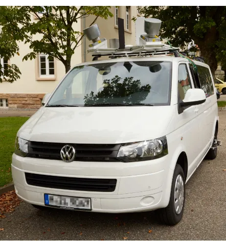
Figure 5. Sensor vehicle used for MLS data recording.
like mobile or terrestrial laser scanners is necessary. The sensor vehicle MODISSA (cf. Figure 5) used to acquire mobile laser scans is augmented with an Applanix POS LV inertial naviga-tion system utilizing two GNSS antennas, an inertial measure-ment unit (IMU) and a distance measuring indicator (DMI). The navigational data is post processed to increase accuracy. Two Velodyne HDL-64E laser scanners are located on the front roof in a 25 degree angle to guarantee good coverage of both road and building facades. Each one of the scanners has a 10 Hz rota-tion rate and collects approximately 1.3 million points per second (Gordon et al., 2015). In terms of accuracy, the standard devia-tion of a single sensor measurement is in the range of about 1.7 cm (Gordon and Meidow, 2013).
TLS The most accurate data source used for the experiments is a Zoller+Fr¨ohlich IMAGER 5003 terrestrial laser scanner based on the phase difference method. With 100 seconds per scan, data collection is slower and more time consuming than MLS, however according to the manufacturer the accuracy is within the range of less than half a centimeter (Zoller+Fr¨ohlich GmbH, 2005). The accuracy also benefits from the fact that the scanner is stationary during a scan.
In a post processing step a fine registration using an ICP algo-rithm is applied to align MLS and ALS, but also to geolocate all TLS scans (cf. Figure 6).
Figure 6. Multiple coregistrated TLS scans.
Standard deviation The accuracy of the data is mainly affected by the process of georeferencing. Therefore the assumed standard
deviation of the 3D point positions is larger than the specific sen-sor error. For the experiments the values in Table 1 are assumed.
data source standard deviation
ALS 0.3 m
MLS 0.3 m
TLS 0.1 m
Table 1. Standard deviation of the utilized data sources. 4.3 Experiments
The method from Section 3. has been evaluated using the data presented above. Different parameters for the model generation were applied, whereby in each set only one parameter or parame-ter pair is modified according to the default values. The different parameter values and their defaults are given in Table 2.
parameter values
sample coverage factor 0.675, 1.645, 1.960, 2.576, 3.29, 5, 10 proportion of outliers 0.05, 0.1,0.2, 0.5, 0.75, 0.9
RANSAC iterations 100
minimal cell size 0.1, 0.2, 0.4, 0.8, 1 m (dstart,dmax) (0.1,2),(0.2,3),(0.5,5),(0.8,6),(1,8),
(2,15),(4,17),(8,33) in points/m2
kmin 3, 5, 7,10, 12, 15, 18, 20, 50
kmax 100, 200, 500, 1000, 5000,10000 minimal variation 0.1, 0.15,0.2, 0.25 Table 2. Evaluated parameter values and theirdefault values.
5. RESULTS AND DISCUSSION
Figure 7 shows exemplary results of the presented model gen-eration algorithm. The building is located in a region where all three types of data (ALS, MLS, and TLS) are available. In such an area a high point density is available and the resulting model shows many details.
The same building is shown on the left side of Figure 8. In the periphery only ALS data are available. Since these data have a far lower point density than the MLS and TLS scans, the polygon model contains less details in these areas and many gaps. The gaps result from the inability of the algorithm to fit a plane due to the sparse point density. Therefore the points in octree cells without plane are also shown.
Changing the parameters of the algorithm could solve this, how-ever this would lead to a loss of details in areas for which data with a high point density are available. These problems could be solved by using different model generation parameters based on the point density in a specific area of the model.
Both examples show some issues with the representation of vege-tation, mainly of trees. The plane fitting is difficult for vegetation since it normally does not consist of planes. This causes our algo-rithm to divide the corresponding octree cells until they are very small. The resulting cells look chaotic and are not optimal with regard to the data compression ratio.
5.1 Data compression ratio
Thedata compression ratiois defined by equation (1). It is the percentage of points represented by planes. The parameterkmax,
dstartanddmaxhave no impact on the data compression ratio.
Figure 7. Exemplary result of the model generation approach.
Figure 8. Larger view of the polygon model extended with points in cells without plane, where the outer areas contain only sparse airborne data.
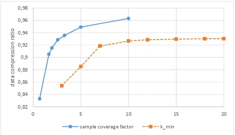
Figure 9 shows the resulting data compression ratio for different values of sample coverage factor andkmin. Both curves show a constant high slope at the beginning that is constantly decreasing at the end. In the middle section the curvatures of both curves are reaching their maximum. For the sample coverage factor this point is reached at a value of2.576,kminshows it at the value7.
As shown in Figure 9, a high sample coverage factor leads to a good compression. But this also results in a high point-to-plane distance threshold, hence small details get lost. So it is more reasonable to set the sample coverage factor to the value2.576(at the point with the highest curvature). This is a trade off between compression ratio and detail preservation.
0,82 0,84 0,86 0,88 0,9 0,92 0,94 0,96 0,98
0 5 10 15 20
d
ata
co
m
p
re
ss
io
n
rati
o
sample coverage factor k_min
Figure 9. Resulting data compression ratio for different values of the sample coverage factor andkmin.
The influence of the minimal cell size and the allowed propor-tion of outliers on the data compression ratio is shown in Fig-ure 10. The maximum of93.4%is reached for a maximal al-lowed proportion of outlier of10%. For higher allowed outlier rates the data compression ratio has a constant descent until it reaches nearly80%with90%allowed outlier rate. With an out-lier proportion of5%the data compression ratio only amounts to 72%.
0 0,1 0,2 0,3 0,4 0,5 0,6 0,7 0,8 0,9 1
0 0,2 0,4 0,6 0,8 1
d
ata
co
m
p
re
ss
io
n
rati
o
proportion of outliers minimal cell size [m]
Figure 10. Resulting data compression ratio for different values of minimal cell size and the proportion of outliers.
5.2 ALS data
The two screen shots in Figure 11 demonstrate the advantage of ALS data: they show the models generated with and without in-cluding it. While the one without airborne scans contains only parts of the building roof, the other one shows the whole roof of the building (cf. Figure 11(b)). This is the main advantage of airborne laser scans.
(a) Without ALS data (b) With ALS data
Figure 11. Impact of ALS data on the generated model.
6. CONCLUSIONS AND FUTURE WORK
Currently our approach uses the database to easily retrieve all data around a given position. These kind of queries are only the simplest way to use a geospatial database. A conceivable option for the future is to utilize more complex queries which for exam-ple retrieve all data along a given path, so that a model for that path could be generated. This could be useful to equip a mobile system with a minimal amount of data required to travel along this path or to visualize a planned path to a user.
The data were assumed to be georeferenced, but this is usually not true for TLS data. Therefore an automatic way of registering TLS with existing MLS or ALS data is required. This needs to take the different precisions of the data sources into account. For the standard deviation of the data to be registered, the accuracy of the georeferenced data needs to be considered. Also the low density of the ALS data poses problems to the model creation. To handle different data densities, further extensions are necessary.
References
Fischler, M. A. and Bolles, R. C., 1981. Random sample consensus: a paradigm for model fitting with applications to image analysis and automated cartography. Communications of the ACM 24, pp. 381– 395.
Gordon, M. and Meidow, J., 2013. Calibration of a multi-beam Laser System by using a TLS-generated Reference. ISPRS Annals of Pho-togrammetry, Remote Sensing and Spatial Information Sciences II-5/W2, pp. 85–90.
Gordon, M., Hebel, M. and Arens, M., 2015. Fast and adaptive surface reconstruction from mobile laser scanning data of urban areas. ISPRS Annals of Photogrammetry, Remote Sensing and Spatial Information Sciences II-3/W4, pp. 41–46.
Hansen, W. v., Michaelsen, E. and Th¨onnessen, U., 2006. Cluster Anal-ysis and Priority Sorting in Huge Point Clouds for Building Recon-struction. In: 18th International Conference on Pattern Recognition (ICPR’06), Hong Kong, China, pp. 23–26.
Hebel, M. and Stilla, U., 2012. Simultaneous Calibration of ALS Systems and Alignment of Multiview LiDAR Scans of Urban Areas. IEEE T. Geoscience and Remote Sensing pp. 2364–2379.
Hoppe, H., DeRose, T., Duchamp, T., McDonald, J. and Stuetzle, W., 1992. Surface Reconstruction from Unorganized Points. In: Proceed-ings of the 19th Annual Conference on Computer Graphics and Inter-active Techniques, SIGGRAPH ’92, ACM, Chicago, USA, pp. 71–78.
Jo, Y., Jang, H., Kim, Y.-H., Cho, J.-K., Moradi, H. and Han, J., 2013. Memory-efficient real-time map building using octree of planes and points. Advanced Robotics 27(4), pp. 301–308.
Lorensen, W. E. and Cline, H. E., 1987. Marching Cubes: A High Reso-lution 3D Surface Construction Algorithm. In: Proceedings of the 14th Annual Conference on Computer Graphics and Interactive Techniques, SIGGRAPH ’87, ACM, Anaheim, USA, pp. 163–169.
Marton, Z. C., Rusu, R. B. and Beetz, M., 2009. On Fast Surface Re-construction Methods for Large and Noisy Datasets. In: IEEE Interna-tional Conference on Robotics and Automation (ICRA), Kobe, Japan, pp. 3218–3223.
Obe, R. and Hsu, L., 2011. PostGIS in Action. In Action, Manning.
Remondino, F., 2003. From point cloud to surface: the modeling and visualization problem. International Archives of Photogrammetry, Re-mote Sensing and Spatial Information Sciences 34(5), pp. W10.
Rusu, R. B. and Cousins, S., 2011. 3D is here: Point Cloud Library (PCL). In: IEEE International Conference on Robotics and Automa-tion (ICRA), Shanghai, China, pp. 1–4.
Vaskevicius, N., Birk, A., Pathak, K. and Poppinga, J., 2007. Fast Detec-tion of Polygons in 3D Point Clouds from Noise-Prone Range Sensors. In: Safety, Security and Rescue Robotics, 2007. SSRR 2007. IEEE In-ternational Workshop on, Rome, Italy, pp. 1–6.
Vosselman, G., Gorte, B. G. H., Sithole, G. and Rabbani, T., 2004. Recog-nising structure in laser scanner point clouds. International Archives of Photogrammetry, Remote Sensing and Spatial Information Sciences 46(8), pp. 33–38.
Wang, M. and Tseng, Y.-H., 2004. Lidar data segmentation and classifi-cation based on octree structure. International Archives of Photogram-metry, Remote Sensing and Spatial Information Sciences 20(B3), pp. 6.