Conference paper

(1)

DEM Construction using DINSAR

Rohit Mangla, Shashi Kumar

mangla1991@gmail.com, shashi@iirs.gov.in

Indian Institute of Remote Sensing (IIRS), ISRO, Dehradun, India

Commission VI, WG VIII/8

KEYWORDS: DEM, DINSAR, Fringes, Decorrelation, Coherence, ALOS PALSAR

ABSTRACT:

A digital elevation model (DEM) is a 3D visualization of a terrain surface. It can be used in various analytical studies such as topographic feature extraction, hydrology, geomorphology and landslides analysis etc. Uttrakhand region is affected with landslides, earthquake and flash flood phenomenon. Hence this study was focused on DEM generation using Differential SAR Interferometry (DINSAR) on ALOS PALSAR dataset. Two Pass DINSAR technique involves one interferometric pair in addition with an external DEM. The external DEM was used as a reference to reduce topographic errors. The data processing steps were image co-registration, interferogram generation, interferogram flattening (Differential Interferogram), interferogram filtering, coherence map, phase unwrapping, orbital refinement and re-flattening and DEM generation. Interferogram fringes observed in forest areas were due to temporal decorrelation and the fringes in mountain regions were obtained due to topography changes (may be due to landslides in rainy season). The range of elevation in generated DEM were 132m to 2823m and Root Mean Square Error (RMSE) error was 36.765159m. The generated DEM was compared with ASTER DEM and variation in height was analyzed. Atmospheric effects were not removed due to geometrical and temporal decorrelation which affect the accuracy.

1. Introduction

In Uttrakhand region, landslides, floods and earthquake are very common phenomenon which leads to loss of lives as well as assets. To analyze these problems, Digital elevation model (DEM) is required. DEM is a 3-D representation of earth surface. It gives elevation value at every (x, y, z) coordinate on the surface. It can be constructed in many ways through stereo pairs (Toutin and Chang 2001), GPS ground data, contour maps (Carrara et al 1997), Lidar data (Axelsson 2000) and SAR Interferometry (Rosen et al 2000). Collection of ground data (DGPS measurements for DEM generation) and contour map generation required much intensive field work and this task is time consuming. For quick detection and prevention from disaster, Synthetic Aperture RADAR (SAR) Interferometry is being used globally.

SAR is an active microwave imaging system. It has its own source of radiation which can be used throughout day and night. SAR sensor can penetrate the cloud cover and can reach the depth in the subsurface. (Richards 2007) SAR Interferometry allows measurement of radiation’s travel path accurately because of coherent nature of microwaves. Measurement of phase difference helps in generation of DEM. ( Semwal 2013)

This study focusses on DEM generation using Differential SAR Interferometry (DINSAR) technique. The main goal was to analyze the accuracy of generated DEM with ASTER DEM. The description of technique is mentioned below.

2. DINSAR Technique

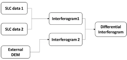
Two Pass Differential Interferometry is an advanced version of SAR interferometry in which two interferograms are generated. One from SLC pair and another interferogram corresponding to surface topography based on external DEM. Finally the difference of phase information of two interferograms are used to generate Differential Interferogram as shown in Fig 1.

Fig 1: Two-Pass DINSAR Technique ( Balaji 2011)

3. Mathematical Background

Consider S1 and S2 are the positions of image radar antenna separated with baseline B as shown in Fig 2. _ℎ and are the parallel and perpendicular baseline respectively. and + � are the ranges from the ground. (Chatterjee, R.)

Fig 2- Geometry of Two-Pass DINSAR ( Marghany 2014)

Phase measurement from S1 position is defined as:

� =4�_� … (2.1)

The International Archives of the Photogrammetry, Remote Sensing and Spatial Information Sciences, Volume XL-8, 2014 ISPRS Technical Commission VIII Symposium, 09 – 12 December 2014, Hyderabad, India

This contribution has been peer-reviewed.

(2)

And from S2 is � =4� +�

� … (2.2)

The phase difference is calculated by subtracting the � from � as shown in equation (2.3)

∆� =4� �_� … (2.3)

Where λ is the wavelength of sensor.

From the cosine law:

+ � = + − 2 ∗ � 90 − � + �

… (2.4)

Where B is the Baseline, θ is the look angle and α is the angle between the parallel baseline _ℎ and original baseline B.

+ � + 2 � = + − 2 ∗ �� − �

… (2.5)

Neglecting ΔR2_{(very small), reshuffle the equation:}

� ≈ sin � − � +� ... (2.6)

Now, the phase of interferogram calculated using equation (2.3) and (2.6) is expressed in equation (2.7)

∆� =4� _� ∗ sin � − � +� ... (2.7)

4. TEST DATA AND STUDY AREA

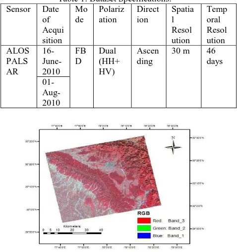
A part of Uttrakhand was selected as study area shown in Fig 3 (LISS III standard FCC) and its central coordinates were 30°13'14.47"N, 77°59'29.29"E. It covers major areas like Dehradun, Rishikesh, Masurrie, Barkot forest and Timli forest range. Two Alos Palsar L-band level 1.1 datasets along with SRTM DEM 90m resolution were used (Rosenqvist, et al 2004). The specifications of datasets are shown below:

Table 1: Dataset Specifications:

Fig 3: Study area (LISS III imagery in standard FCC)

5. METHODOLOGY

The methodology adopted for the research work is shown below in Fig 4.

Fig 4: Flow diagram of Methodology

Baseline Estimation:

It provides information about baseline values and orbital parameters of interferometric pair. This information is not used for DEM generation but provides the feasibility of data.

Co-registration:

Co-registration is defined as a process of superimposing two or more SAR images in the slant range geometry. External DEM is used for this purpose. (Li and Bethel 2008)

Interferogram Generation:

Each pixel of SLC image has amplitude as well as phase information. The interferogram is generated by Hermition product of each pixel between two co-registered images. The formula is shown below in equation (5.1):

� = � ∗ ∗ _{… (5.1)}

Where � is the pixel value of interferogram, � and are the pixel value of master and slave image respectively.

Phase can be calculated using the equation (5.2):

� = tan− � ��

ground displacement between two SAR images.

(3)

Interferogram Flattening (Differential Interferogram): The phase calculated in interferogram is affected due to earth curvature. The process of its removal is called Interferogram flattening. This provides us with fringes which are related to change in displacement (if any), elevation, noise and atmospheric effects. The flat phase can be estimated as shown below:

∆� � = 4�_� [ sin � − � − sin � − � ] … (5.4)

Where �= look angle to each point in the image assuming zero local height

Interferogram Filtering and Coherence Generation: Filtering reduces the noise and smoothens the interferogram. Coherence map is generated from the filtered interferogram. It measures the degree of similarity between two pixels. The mathematical formula is given below: (Fletcher, K. 2007)

� = Σ�� ∗

√Σ�|� | √Σ�| | … (5.5)

Where N is the no of pixels, M1 is master image, S1 is the slave

image and S1* is the complex conjugate of slave image.

The significance of coherence map is to determine the quality of interferometric pair. Low coherence means the data is not suitable for DEM generation.

Phase Unwrapping:

The range of interferogram phases is (–π, π) only. This process is used to add the correct multiple of phases which resolves the 2π ambiguity. (Reigber and Moreira 1997)

� � = � � + 2 � … (5.6)

Where � _� is the wrapped phase, � _� is unwrapped phase and n is a positive integer.

Orbital refinement and re-flattening:

This step refines the orbit values, removes the phase ramps and calculates the phase offset values. This is compulsory step for DEM generation. Ground control point file is required to execute this step.

DEM Generation:

The calibrated and unwrapped phase value is converted into height value and geocoded into map projection. The height value is calculated using normal baseline method expressed in equation (5.7).

∆ℎ = � � �_{4� B⊥} ∗ ∆� … (5.7)

Coherence image is also geocoded after this step.

6. RESULT AND DISCUSSION

Baseline: The normal baseline of data-pair is less than the critical baseline as shown in Table 1. It means data pair is suitable for DEM generation.

Table 1: Baseline Data

Pair

Baseline 2π ambiguity

Normal Critical Temporal Height

Jun-Aug

767.061 6525.452 46 days 83.497

Interferogram Generation:

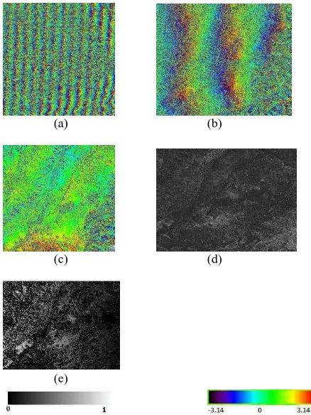
Fringes absorbed in the image are the phase changes due to topography, atmospheric effects, noise and displacement (if any) shown in Fig 4(a).

Interferogram Flattening:

Phase difference due to curvature of earth was removed. Phase discontinuity can be seen as contour lines as shown in Fig 4(b).

Filtered Interferogram:

Interferogram fringes in forest area were observed due to temporal decorrelation and in mountain regions it was observed due to change in topography as shown in Fig 4(c).

Coherence Map:

Bright pixels can be seen in settlement area showing high correlation whereas dark pixels can be noticed in forest areas showing low correlation in Fig 4(d). Low correlation may be due to shift in orientation of leaves or due to change in moisture at the time of data acquisition.

Wrapped Phase Image:

Grey level continuity observed in wrapped image as seen in Fig 4(e) shows that the phase information is relative and calibrated in order to convert it into height.

(a) (b)

(c) (d)

(e)

Fig 4: (a) Interferogram (b) Flattened Interferogram (c) filtered Interferogram (d) coherence map (e) Wrapped Phase

DEM Generation:

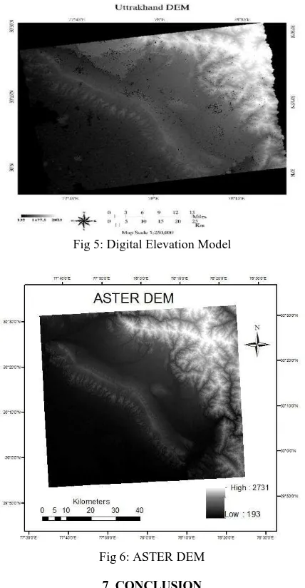
Generated DEM was of 25m resoution having elevation values between 132m to 2823m as shown in Fig 5. The RMSE error was calculated using three degree polynomial function was 36.765159m. The newly constructed DEM was than compared with ASTER DEM having elevation values between 193m to 2731m as shown in Fig 6 and it was found to have very less variation in settlement areas and high variation in mountaneous and forest areas.

(4)

Fig 5: Digital Elevation Model

Fig 6: ASTER DEM

7. CONCLUSION

The goal of this study was to generate the DEM using Differential SAR Interferometry. Two dual polarized ALOS Palsar dataset were used along with 90m resolution external DEM (SRTM). From the results, RMSE errors were found very less in urban areas due to high correlation whereas more errors were obtained in mountainous regions (may be due to landslides in rainy season) and forest regions due to temporal decorrelation. These errors could be further reduced by using 30m resolution external DEM.

Atmospheric effects were not removed with this technology. Further improvements can be done using PSINSAR and SqueeSAR technologies.

REFERENCES

Axelsson, P. (2000) “DEM generation from laser scanner data using adaptive TIN models” InternationalArchives of Photogrammetry and Remote Sensing. Vol. XXXIII, Part B4. Amsterdam.

A. Rosenqvist, M. Shimada and M. Watanabe (2004). “ALOS PALSAR: Technical outline and mission concepts,” in 4th

International Symposium on Retrieval of Bio-and Geophysical Parameters from SAR Data for Land Applications, pp. 1–7.

Balaji, M. P. (2011)“Estimation and Correction of Tropospheric and Ionospheric Effects on Differential SAR Interferograms” M Sc Indian Inst. Remote Sens. IIRS Int. Inst. Geoinformation Sci. Earth Obs. ITC,.

Carrara, A., Bitelli, G., Carla, R. (1997) “Comparison of techniques for generating digital terrain models from contour lines” International Journal of Geographical Information Science, vol 11, issue 5.

Fletcher, K. (2007) “InSAR principles: guidelines for SAR interferometry processing and interpretation.” Noordwijk, the Netherlands: ESA Publications Division, ESTEC, 2007.

Li, F. K., Bethel, J. (2008). “Image Co-registration in SAR Interferometry" The International Archives of Photogrammetry, Remote Sensing and Spatial Information Sciences, volume XXXVII, part 1, Beijing, China.

Marghany, M. (2014) “A Three-dimensional of Coastline Deformation using the Sorting Reliability Algorithm of ENVISAT Interferometric Synthetic Aperture Radar”

Advanced Geoscience Remote Sensing, Prof. Maged Marghany (Ed.), ISBN: 978-953-51-1581-6, InTech, DOI: 10.5772/58571.

Semwal, P. (2013). “Study of slow moving Landslides using SAR Interferometry Technique,” Andhra University, Indian Institute of Remote Sensing, Dehradun.

Reigber, A. and Moreira, J. (1997). “Phase Unwrapping by Fusion of Local and Global Methods.” Geoscience and Remote Sensing, 1997, IGARSS 97, Singapore 3-8th August, pp. 869- 871, Remote Sensing- A Scientific Vision for Sustainable Development 1997 IEEE International.

Richards, M. (2007). “A Beginner's Guide to Interferometric SAR Concepts and Signal Processing.” IEEE A & E Systems magazine, vol. 22, no 9, ISBN 0018-9251

Rosen, P.A., Hensley, S., Joughin, I.R., (2000). “Synthetic Aperture Radar Interferometry” Proceedings of the IEEE, 88 (3): 333-382.

R. S. Chatterjee, “Baiscs of InSAR and DInSAR: Concepts and Applications.”

Toutin, T., Cheng, P., (2001) “DEM Generation with ASTER Stereo Data” EOM Current Issues.