SPATIO-TEMPORAL PATTERN ANALYSIS FOR REGIONAL CLIMATE CHANGE
USING MATHEMATICAL MORPHOLOGY
M. Dasa, S. K. Ghosha,∗
a
School of Information Technology, Indian Institute of Technology Kharagpur - [email protected], [email protected]
KEY WORDS:Climate Change, Spatio-temporal Pattern, Mathematical Morphology, Directional Granulometry, Multifractal Analysis
ABSTRACT:
Of late, significant changes in climate with their grave consequences have posed great challenges on humankind. Thus, the detection and assessment of climatic changes on a regional scale is gaining importance, since it helps to adopt adequate mitigation and adaptation measures. In this paper, we have presented a novel approach for detecting spatio-temporal pattern of regional climate change by exploiting the theory ofmathematical morphology. At first, the various climatic zones in the region have been identified by using multifractal cross-correlation analysis(MF-DXA) of different climate variables of interest. Then, thedirectional granulometrywith four different structuring elements has been studied to detect the temporal changes in spatial distribution of the identified climatic zones in the region and further insights have been drawn with respect tomorphological uncertainty indexandHurst exponent. The approach has been evaluated with the daily time series data ofland surface temperature(LST) andprecipitation rate, collected fromMicrosoft Research - Fetch Climate Explorer, to analyze the spatio-temporal climatic pattern-change in theEasternandNorth-Easternregions of Indiathroughout four quarters of the 20th century.
1. INTRODUCTION
Modeling climate change has become one of the major research issues as it has serious consequences on human life and eco-hydrological processes (Wu et al., 2013). The key challenges here stem from the complex nature of climate data itself. It is because the individual climate variables, governing a climate regime, show very distinctive pattern of change, and the change-pattern also varies from one region to another region throughout the world. Therefore, the regional analysis of climatic pattern change is of utmost significance, particularly for planning adequate mitigation and adaptation measures.
However, the literature mostly concentrates onimpact of climate change(Li et al., 2012, Lehodey et al., 2014), than on analy-sis of climate change pattern. Moreover, the majority of existing works on change pattern analysis (Somot et al., 2008, Gibelin and D´equ´e, 2003, Mahlstein and Knutti, 2010) are based onglobal climate modelsthat suffer from the limitations in computing power as well as in proper scientific understanding of physical processes.
In the present work, we have proposed a novel approach for an-alyzing climate change pattern on regional scale. This is adata driven approach, based on the theory ofmathematical morphol-ogy, and hence, it intuitively overcomes the inherent limitations of the aforesaid methods. Although thehigh dimensionalityof climate data becomes a major issue in data driven approach, the problem has been tackled by defining a new low-dimensional data set by utilizingmultifractal detrended cross correlation analysis (MF-DXA).
1.1 Contributions
The proposed approach consists of three main steps: i)to iden-tify the various climate zones in the study region using a spatio-temporal data mining technique as proposed in (Das and Ghosh, 2015);ii)to detect any regional change in the identified climate zones during each considered time period by utilizing the basic operators inmathematical morphology; iii)to characterize the
∗Corresponding author, Tel: +91 3222-282332
pattern of climate change, occurred if any, by means of granu-lometric analysiswith fourdirectional structuring elements, ori-ented inNorth-South(N-S),East-West(E-W),NorthEast-South West(NE-SW), andNorthWest-SouthEast(NW-SE) directions re-spectively. The approach has been evaluated empirically with the land surface temperatureandprecipitation ratedata sets1of 20th century, collected from 240 different locations over all the 12 states in entireEasternandNorth-Eastern regionsofIndia. The high resemblance of the simulated climate-change-pattern with that really encountered during the hundred-year period (1901-2000) in the study area, proves and validates the efficacy of our proposed approach. Thus, the main contributions of this work can be summarized as follows:
• Proposing an approach for analyzing spatio-temporal pat-terns in regional climate change on the basis ofdirectional granulometry.
• Exploring the theory ofmathematical morphologyand mul-tifractal analysisin climatological study.
• Experimenting with hundred-year data ofland surface tem-peratureandprecipitationtime series over 240 locations on 0.5◦
×0.5◦
grid in the study region.
• Drawing insights regarding the pattern of regional climate change usingmorphological uncertainty indexandHurst ex-ponent.
• Verifying the effectiveness of the proposed approach by an empirical study of analyzing climate change pattern during the 20th century inEasternandNorth-Eastern India.
The rest of the paper is organized as follows: In section 2., we have a review of some related works. Section 3. briefly describes the theoretical background behind the work. The proposed ap-proach for climate change pattern detection and analysis has been illustrated in section 4. The results of simulation have been re-ported in section 5., along with a brief description of the study
A decision support system has been proposed in (Wilby et al., 2002) for assessing regional climate change using a robust sta-tistical downscaling technique. The use of stasta-tistical downscal-ing helped in rapid development of scenarios with daily surface weather variables under current and future regional climate forc-ing. The technique proposed in (McCallum et al., 2010), is based on the sensitivity analysis of climate variables using a soil-vegeta tion-atmosphere-transfer model. The approach helped to deter-mine the importance of various climate variables in regional change analysis. Few more relevant studies can be found in (Maurer et al., 2007, Li et al., 2012, Lehodey et al., 2014). However, these works are mainly centered on the analysis ofimpact of climate change, rather than on the analysis ofclimate change pattern.
On the other hand, the existing research works onregional cli-mate change pattern analysis are mainly based on the various global circulation models or GCMs (Nobre et al., 1991, Gibelin and D´equ´e, 2003, Somot et al., 2008, Mahlstein and Knutti, 2010). For example, Nobre et al. in (Nobre et al., 1991) has used a cou-pled numerical model for a global as well as regional assessment of climate change due to Amazonian deforestation. A sea atmo-sphere Mediterranean model has been proposed in (Somot et al., 2008), where global atmosphere model has locally been coupled with regional ocean circulation model to study the climate evo-lution in the Mediterranean region. A number of global coupled atmosphere ocean general circulation models (AOGCMs)have been used in (Mahlstein and Knutti, 2010) to identify the regional climate-change-pattern through a cluster analysis. A variable res-olution atmospheric model has been used to simulate the mean sea surface temperature and precipitation field in (Gibelin and D´equ´e, 2003). However, all these works, being based on global and/or regional climate models, suffers from the limitations of high computing power requirementsandincomplete scientific un-derstanding of physical processesin climatology, as mentioned earlier.
Our proposed approach forregionalclimate change pattern anal-ysis is adata driven approach, and it attempts to overcome the inherent limitations of the existing approaches based on GCMs. Besides, the problem withhigh dimensionalityof climate data, that becomes a major issue in data driven approaches, has been handled here, by defining a new low-dimensional data set by utilizingmultifractal detrended cross correlation analysis (MF-DXA). Moreover, the novelty of the proposed method lies in ana-lyzing the regional climate change considering thegeometric as-pectsof spatial distribution of various climate zones in the region. To achieve this goal, we have utilized the theory ofmathematical morphologyfollowed bygranulometric analysis.
3. BACKGROUND
This section provides a very brief description of the theoretical background behind our approach, namely, definitions of some ba-sic morphological operators, and multifractal analysis.
by:
A⊖B={a−b:a∈A, b∈B}= \
b∈B
A−b (1)
Dilation: DilationofAbyBincreases the size ofA, which is shown in eq. (2)
A⊕B={a+b:a∈A, b∈B}= [
b∈B
Ab (2)
Opening:Openingtransformation of the setAbyBis given by:
A◦B= (A⊖B)⊕B (3)
Multi-scale Opening:Multi-scale morphological openingcan be performed by increasing the size ofBas given in eq. (4)
A◦nB= (A⊖nB)⊕nB (4)
Closing: Similarly,closing transformation ofA by B can be given as follows.
A•B= (A⊕B)⊖B (5)
Multi-scale Closing: Multi-scale morphological closingcan be performed by increasing the size ofBas shown below:
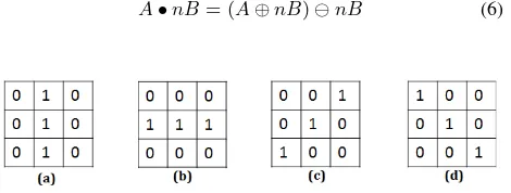
A•nB= (A⊕nB)⊖nB (6)
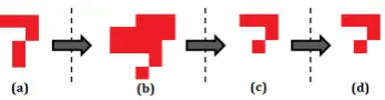
Figure 1. Four directional structuring elements: (a)North-South (N-S), (b)East-West(E-W), (c)NorthEast-SouthWest(NE-SW), (d)NorthWest-SouthEast(NW-SE)
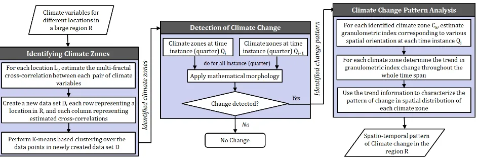
im-Figure 2. Flow diagram of the proposed approach for regional analysis of spatio-temporal pattern in climate change
age) can be defined as follows:
H(A/B) =− where,Card(.)is the cardinality of the set, andN is the mini-mum positive integern, such that(A◦nB)6=φand(A◦(n+ 1)B) =φ.
In case of directional granulometry (Vardhan et al., 2013), the structuring elementBis a directional structuring element (exam-ple shown in Figure 1).
3.2 Fractals and Multifractals
Fractals are the never-ending, self-similar patterns that repeat them-selves at different scales (Falconer, 2004). These can either be mathematical or natural objects, whose complexity are quantified in terms of a special measure calledfractal dimension. Some of the popular definitions of fractal dimensions are: Hausdorff di-mension, Box-counting dimension, and Information dimension. In general, fractal dimensions are determined from the regression lines overlog vs. logplots ofsize (or, change in detail) vs. scale. For example, the box-counting dimension (DB), as defined
be-low, is estimated as the exponent of a power law.
DB = lim ǫ→0
logN(ǫ)
log (1/ǫ) (9)
where,N(ǫ)is the number of boxes of side lengthǫrequired to cover the fractal object.
There are some objects which cannot be described in terms of a single scaling exponent (fractal dimension), and a multitude of fractal dimensionsare required to characterize them properly. These are calledmultifractals. Unlike fractals, the self-similarity in multifractals are scale-dependent. Some common multifrac-tals, found in nature, are the various climatic time series like air temperature, precipitation, humidity etc.
3.2.1 Multifractal Detrended Cross-Correlation Analysis (MF-DXA): TheMF-DXAmethod as proposed by (Zhou, 2008) is a multifractal modification of thedetrended cross-correlation anal-ysis (DXA), and quantifies the long-range cross-correlations be-tween two non-stationary time series. Long-range cross-correlations between two series imply that each series has long memory of its
own previous values and that of the other series also. If the large and small covariance scales differently, then there will be a sig-nificant dependence between detrended cross-covarianceF(q, l) and scale lengthl, for different positive and negative values ofq, which characterizes the multifractality of the series in terms of generalized Hurst exponentsh(q)(also calledmultifractal scal-ing exponents). The detailed calculations involved in various steps ofMF-DXAmethod can be found in (Zhou, 2008).
The present work usesMF-DXAto detect the climate zones in a large region based on similarity in cross-correlation pattern among different locations in the region.
4. METHODOLOGY
Figure 2 presents the basic block diagram of the proposed ap-proach for analyzing spatio-temporal pattern in regional climate change. The system takes as input the historical time series data of various climate variables for different locations in the study region, and finally generates insights regarding the pattern of cli-mate change throughout the past years. As depicted in the figure, the entire system comprises three major steps, namely, (A) Iden-tifying climate zones, (B)Detection of climate change, and (C) Change pattern analysis.
4.1 Identifying Climate Zones
The objective here is to capture the long-range cross-correlation between each pair of climate variablesuandvover different time scale to characterize the climate pattern of different locations of a regionR, and then to identify the various climate zones inRon the basis of similarity in spatio-temporal pattern among different locations. The whole estimation is performed in two phases: i) Multifractal cross-correlation analysis, andii) Data clustering.
4.1.1 Multifractal cross-correlation analysis: In this phase, a new database, attributing each location, is created. Each tu-ple/row in the database corresponds to a particular location in the regionR, and each field/column becomes the multifractal scaling exponents, obtained from multifractal cross-correlation analysis using MF-DXA as follows:
huv(q) =
log [Fuv(q, l)]
logl +c (10)
where,cis a constant term. Here,Fu,v(q, l)is the q-th order
detrended covariance betweenuandvover a time scale length of l.huv(q)is also termed asgeneralized Hurst exponent.The new
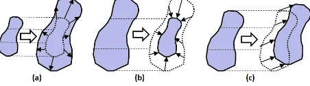
The main purpose of this step is to detect whether any climatic change has occurred in a region during a particular time period. In general, the spatio-temporal change pattern can broadly be classified into geometric changeand thematic change (Ping et al., 2008). The geometric change pattern mainly impliesgrowth, shrinkage, anddriftof spatial orientation (Figure 3). In our work, we have considered the first two as the pattern of change. As a growth pattern we have consideredspatial expansion, and as a shrinkage pattern we have consideredspatial contraction. The other kinds of growth and shrinkage can be spatial mergeand splitrespectively.
Figure 3. Change pattern: (a)Growth (expansion), (b)Shrinkage (contraction), (c)Drift
LetCt=Set of all locations under a particular climate zoneCat
a time instantt,C(t+n)=Set of all locations under a particular
climate zoneC at a time instant(t+n), Then the conditions forgrowth,shrinkage, andno-changein spatial distribution pat-tern ofCcan be defined asCt ⊂ C(t+n), Ct ⊃ C(t+n), and
Ct=C(t+n)respectively. In our proposed approach, the
spatio-temporal pattern of climate change has been detected on the basis of above conditions and utilizing morphological operators as fol-lows:
where,Bis a structuring element,Card(x)is the cardinality of setx, andNmaxis a positive integeri, such that either(Ct◦(i+
1)B)or(C(t+n)◦(i+ 1)B)becomesφ.
A climate zone is treated to bespreading (growing)if it shows growth pattern during most of the instances in a time duration. Similar decision can be made regardingshrinkageandno-change of a zone. As explained in Figure 2, if no change is detected, the process stops, and no further analysis is performed.
Orient(Ct) = Dir(Bi) :max(H(Ct/Bi)),∀i (11)
where,Dir(Bi)
is the direction of thei-th structuring element Bi
, and theH(Ct/Bi)is thegranulometric index (uncertainty
index)corresponding toBi, as mentioned in section 3..H(Ct/Bi)
is calculated in following manner:
H(Ct/Bi) =−
where,nis the size of structuring element, andNmaxis a positive
integer such that(Ct◦NmaxB)6=φand(Ct◦(Nmax+1)B) =
φ.
The spatial distribution (orientation) of each climate zone, thus calculated for each time instant, eventually help to achieve in-sights on the direction of growing (or shrinkage).
4.3.2 Change-pattern categorization: This phase determines the change in spatial orientation of each climate zone from one time instant to another. In other words, it helps to determine the direction of growing (or shrinkage) of the climate zones in a re-gion.
Once the spatial distribution of each climate zone at each time instant is obtained, the characteristics of each pattern is analyzed in terms oftrend in temporal change of granulometric indices. Three types of pattern characteristics have been considered: i) Extinguishing,ii) Evolving, and iii) Stationary. It is evident from eq. 11 that, the more is the value of granulometric index, the higher is the tendency to be oriented in the respective direction. Based on this observation, the pattern of change during a given time period is characterized as follows:
Let,Ctbe a climate zone (set of locations), orientated towardsBi
at time instantt, andC(t+n) be the same zone with orientation
towardsBj
at time instant(t+n). Also let, the linear trend of change in granulometric index corresponding toBi andBj
Figure 4. Study area: (a)EasternandNorth-Easternregion of India, (b)240 locations on a0.5◦ ×0.5◦
grid, (c) Identified climate zones in the study region
• moreover, if(Bi6=Bj), the orientation ofC
tchanges from
Dir(Bi)toDir(Bj).
Now, if a climate zone shows a growing pattern along with an extinguishing characteristics, then this indicates its growth not only in its current orientation, but in the opposite direction also. Again, if the zone shows a shrinking pattern along with an evolv-ing characteristics, then this indicates shrinkage in the opposite direction of its current orientation. In the similar fashion, sev-eral other inferences can be drawn regarding the spatio-temporal pattern of regional climate-change.
5. EMPIRICAL EVALUATION
In this section we have evaluated our proposed approach of cli-mate change-pattern analysis, using an empirical study.
5.1 Data set and Study area
The experimentation has been performed using the daily time se-ries data of two major climate variables, namely, land surface temperatureand precipitation rate, collected from theEastern andNorth-Easternregion ofIndia. As depicted in Figure 4(a), this region of India consists of 12 states. The spatio-temporal data has been collected from 240 different locations on a0.5◦
×0.5◦ grid over all these states as pointed in Figure 4(b). The data has been obtained from theFetchClimate Explorersite (Microsoft-Research, 2014) for a duration of 100 years (1901-2000), in the 20th century.
5.2 Experimental Setup
The entire experiment has been carried out using MATLAB 7.12.0 (R2011a) in Windows 2007 (32-bit Operating System, 2.40 GHz CPU, 2.00 GB RAM), and R-tool version 3.1.1 (32 bit). Here, each quarter of the century has been treated as a time instant, and the daily time series data of each climate variable has been averaged over 25-year period to get the representative series for respective quarter.
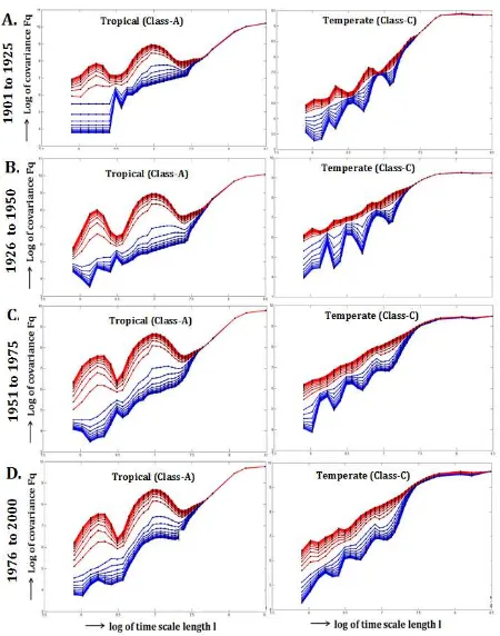
During the climate zone identification step, the q-th order de-trended covariance (Fuv(q, l)) vs. scale size (l) has been
stud-ied for identifying the pattern of multifractal correlation between the time series oftemperature(u) andprecipitation rate(v). The study reveals that the multifractal nature of the correlation pattern changes with the climate pattern of a location. The pattern infor-mation is then captured in terms of multifractal scaling exponents huv(q)(generalized Hurst exponent, estimated as the slope of the
log-log plot for each values ofq), and is utilized to cluster the locations into climate zones. The identified climate zones (Tem-perateandTropical) for all the four quarters of the 20th century, and their corresponding patterns of multi-fractal cross-correlation have been depicted in Figure 4(c) and Figure 5 respectively.
Figure 5. Multifractal cross-correlation pattern of different cli-mate zones
(c)1951-1975, (d)1976-2000
Figure 7. Change in spatial distribution of theTemperate climate zone (C): (a)1901-1925, (b)1926-1950, (c)1951-1975, (d)1976-2000
Figure 8. Change in spatial distribution of theTropical climate zone (A2) in North-Eastern India: (a)1901-1925, (b)1926-1950, (c)1951-1975, (d)1976-2000
Figure 9. Confusion matrices obtained in climate zone identifica-tion
5.3 Performance Evaluation
The accuracy ofclimate zone detection has been measured in comparison with theworld map of K¨oppen-Geiger classification (Rubel and Kottek, 2010). Two different performance measures (Overall Accuracy (OA), andFalse Alarm Ratio (F AR)), as shown
in Table 1, have been used for quantitative evaluation. The val-ues of the different parameters are obtained from the confusion matrices (Figure 9) achieved for each quarter of the century.
Performance of climate change pattern detection and analysis has been studied empirically in comparison with the actual cli-mate change encountered during the whole century as shown in the Figure 10.
OA= T P+T NT P++F PF N+F N ;F AR= T PF P+F P
T P=True Positive;T N=True Negative F P=False Positive;F N=False Negative
6. DISCUSSION
The observations from the empirical study are as follows:
• From the Figures 9 and 4(c), it is evident that two major types of climate zones, namely, Tropical and Temperate, have been identified in the first step, and highly resemble with that in theworld map of K¨oppen-Geiger classification (Rubel and Kottek, 2010).
• The high values ofoverall accuracy(OA), and a very low
false alarm ratio (FAR), as shown in Table 1 also ensures the efficiency of our approach in climate zone identification.
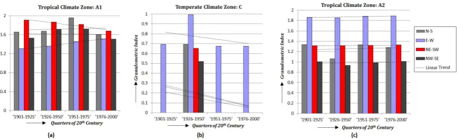
From the graphical plot of granulometric indices (refer Figure 11), the following inferences can be drawn regarding the perfor-mance of the proposed approach in climate-change-pattern anal-ysis:
• The tropical zone A1 (refer Figure 11(a)) in Eastern In-dia shows a decreasing trend of granulometric index (un-certainty index) corresponding to its current direction (NE-SW). Since, in the change detection step the zone has shown a shrinking pattern, it ensures the direction of shrinkage to be inNE-SW. Hence, there must exist a current tendency to be oriented in a different direction. The same is evident from the increasing trend of uncertainty index correspond-ing to E-W direction (Figure 11(a)).
• It may be noted from Figure 11(b) that, the temperate zone Cshows a decreasing trend of granulometric index (uncer-tainty index) corresponding to its currently prevailing di-rection (E-W). Since, in the change detection step the zone shows a growing pattern, there must exist a current tendency to grow in the opposite direction (N-S) as well. The same is evident from the actual change in climate as shown in Figure 10(b).
• Therefore, it can be concluded from the above two points that, the type of climate in the North-East part of Eastern India is being changed from tropical to temperate. Thus, the locations in this part of India is going to encounter more hot summer, and a long winter. The same is true for middle East part of North-Eastern India also.
Figure 10. Spatio-temporal change in climate zones during 20th century: (a)Tropical climate zone (A1) in Eastern India, (b)Temperate zone (C), (c)Tropical climate zone (A2) in North-Eastern India
Figure 11. Change inGranulometric indices(corresponding to various structuring elements) throughout 20th century: (a)Tropical climate zone (A1) in Eastern India, (b)Temperate zone (C), (c)Tropical climate zone (A2) in North-Eastern India
The fifth assessment report ofIPCC(IPCC, 2013) supports our outcomes, and demonstrates its efficacy in regional analysis of climate change pattern.
7. CONCLUSIONS
This work presents a data driven approach to detect and ana-lyze the regional climate-change pattern on the basis oftemporal change in spatial orientationof various climate zones in the re-gion. It has exploited the principles ofmultifractal analysisand mathematical morphologyto identify the climate zones, and to perform thegranulometric analysiswith fourdirectional struc-turing elements. A case study has been performed with the tem-peratureandprecipitationdata ofEasternandNorth-Eastern re-gion ofIndia, to analyze the spatio-temporal climate-change dur-ing 1901-2000. ANE-SWshrinkage oftropical climate zonein the Eastern India, and a growth of temperate climate zone in both E-W and N-S direction have been detected. The high resem-blance of the simulated climate-change-pattern with that really encountered during the whole century, proves and validates the effectiveness of applyingmultifractalandmorphological analy-sisin climate-change-study. This work has considered two basic change patterns: growth and shrinkage, in spatial distribution of climate zones. In future, the work can be extended to deal with the other kinds of patterns like merging, splitting, and drifting or a combination of them.
REFERENCES
Das, M. and Ghosh, S. K., 2015. Detection of climate zones using multifractal detrended cross-correlation analysis: A spatio-temporal data mining approach. In: Eighth International Confer-ence on Advances in Pattern Recognition (ICAPR), 2015,IEEE, pp. 1–6.
Falconer, K., 2004.Fractal geometry: mathematical foundations and applications. John Wiley & Sons.
Gibelin, A.-L. and D´equ´e, M., 2003. Anthropogenic climate change over the mediterranean region simulated by a global vari-able resolution model.Climate Dynamics20(4), pp. 327–339.
IPCC, 2013. Climate Change 2013: The Physical Science Ba-sis.http://www.ipcc.ch/report/ar5/wg1/docs/. [Online; Accessed 18-Aug-2014].
Lehodey, P., Senina, I., Nicol, S. and Hampton, J., 2014. Mod-elling the impact of climate change on south pacific albacore tuna. Deep Sea Research Part II: Topical Studies in Oceanography.
Li, D. H., Yang, L. and Lam, J. C., 2012. Impact of climate change on energy use in the built environment in different climate zones–a review.Energy42(1), pp. 103–112.
Mahlstein, I. and Knutti, R., 2010. Regional climate change patterns identified by cluster analysis. Climate dynamics35(4), pp. 587–600.
Maurer, E. P., Brekke, L., Pruitt, T. and Duffy, P. B., 2007. Fine-resolution climate projections enhance regional climate change impact studies. Eos, Transactions American Geophysical Union 88(47), pp. 504–504.
McCallum, J., Crosbie, R., Walker, G. and Dawes, W., 2010. Im-pacts of climate change on groundwater in australia: a sensitiv-ity analysis of recharge.Hydrogeology Journal18(7), pp. 1625– 1638.
Microsoft-Research, 2014. FetchClimate. http://research. microsoft.com/en-us/um/cambridge/projects/
Serra, J., 1986. Introduction to mathematical morphology. Com-puter vision, graphics, and image processing35(3), pp. 283–305.
Somot, S., Sevault, F., D´equ´e, M. and Cr´epon, M., 2008. 21st century climate change scenario for the mediterranean using a coupled atmosphere–ocean regional climate model. Global and Planetary Change63(2), pp. 112–126.
Vardhan, S. A., Sagar, B. D., Rajesh, N. and Rajashekara, H., 2013. Automatic detection of orientation of mapped units via di-rectional granulometric analysis. Geoscience and Remote Sens-ing Letters, IEEE10(6), pp. 1449–1453.
Wilby, R. L., Dawson, C. W. and Barrow, E. M., 2002. Sdsma de-cision support tool for the assessment of regional climate change impacts. Environmental Modelling & Software17(2), pp. 145– 157.
Wu, F., Wang, X., Cai, Y. and Li, C., 2013. Spatiotemporal analy-sis of precipitation trends under climate change in the upper reach of mekong river basin.Quaternary International.