VALIDATION OF BIM COMPONENTS BY PHOTOGRAMMETRIC POINT CLOUDS
FOR CONSTRUCTION SITE MONITORING
S. Tuttasa,∗, A. Braunb, A. Borrmannb, U. Stillaa a
Photogrammetry & Remote Sensing, TU M¨unchen, 80290 M¨unchen, Germany - (sebastian.tuttas, stilla)@tum.de bComputational Modeling and Simulation, TU M¨unchen, 80290 M¨unchen, Germany
-(alex.braun, andre.borrmann)@tum.de
Commission III, WG III/4
KEY WORDS:photogrammetric point cloud, construction site monitoring, 3D building model, BIM
ABSTRACT:
Construction progress monitoring is a primarily manual and time consuming process which is usually based on 2D plans and therefore has a need for an increased automation. In this paper an approach is introduced for comparing a planned state of a building (as-planned) derived from a Building Information Model (BIM) to a photogrammetric point cloud (as-built). In order to accomplish the comparison a triangle-based representation of the building model is used. The approach has two main processing steps. First, visibility checks are performed to determine whether or not elements of the building are potentially built. The remaining parts can be either categorized as free areas, which are definitely not built, or as unknown areas, which are not visible. In the second step it is determined if the potentially built parts can be confirmed by the surrounding points. This process begins by splitting each triangle into small raster cells. For each raster cell a measure is calculated using three criteria: the mean distance of the points, their standard deviation and the deviation from a local plane fit. A triangle is confirmed if a sufficient number of raster cells yield a high rating by the measure. The approach is tested based on a real case inner city scenario. Only triangles showing unambiguous results are labeled with their statuses, because it is intended to use these results to infer additional statements based on dependencies modeled in the BIM. It is shown that the labelbuilt
is reliable and can be used for further analysis. As a drawback this comes with a high percentage of ambiguously classified elements, for which the acquired data is not sufficient (in terms of coverage and/or accuracy) for validation.
1. INTRODUCTION
1.1 Motivation
A Building Information Model (BIM) contains the 3D geometry of a building, as well as the process information of the construc-tion what makes the 3D to a 4D building model. For progress monitoring, the planned states (as-planned) of the construction have to be validated against the actual state (as-built) at a cer-tain time step. Today this is a primarily manual process which is usually based on 2D plans. Because of the dynamic process sequences of construction projects, it has to be assumed that the actual execution of the construction work differs strongly from the planning at the beginning of the project. Reasons for this gap are, among others, delivery delays, delays in construction and the strong dependencies between the single processes. For detect-ing deviations from the schedule as quickly as possible, allow-ing a prompt response, an automatic construction progress mon-itoring system is desirable, which works directly with the BIM. The detected deviations lead to modifications of the schedule and the following processes modeled in the BIM. Difficulties on con-struction sites for the monitoring arise because of occlusions, the occurrence of various temporal objects or the limited accessibility of acquisition positions. The goal is to derive a statement about the status of a certain building element at a certain time step based on the obtainable data. Therefore a measure which can cope with occlusions and noisy sections of the point cloud is needed.
1.2 Related Work
The basic acquisition techniques for construction site monitoring are laser scanning and image-based/photogrammetric methods.
∗Corresponding author
monitoring is given by (Rankohi and Waugh, 2014). (Ibrahim et al., 2009) introduce an approach with a single, fixed camera. They analyze the changes of consecutive images acquired every 15 minutes. The building elements are projected to the image and strong changes within these regions are used as detection criteria. This approach suffers from the fact that often changes occur due to different reasons than the completion of a building element. (Kim et al., 2013a) also use a fixed camera and image processing techniques for the detection of new construction elements. The results are used to update the construction schedule. Since many fixed cameras would be necessary to cover a whole construction site, more approaches, like the following and the one presented in this paper, rely on images from hand-held cameras to cover the complete construction site.
In contrast to a point cloud received from a laser scan a scale has to be introduced to a photogrammetric point cloud. A possibility is to use a stereo-camera system, as done in (Son and Kim, 2010), (Brilakis et al., 2011) or (Fathi and Brilakis, 2011). (Rashidi et al., 2014) propose to use a colored cube with known size as target, which can be automatically measured to determine the scale. In (Golparvar-Fard et al., 2011a) image-based approaches are compared with laser-scanning results. The artificial test data is strongly simplified and the real data experiments are limited to a very small part of a construction site. In this case no scale was introduced to the photogrammetric measurements leading to accuracy measures which are only relative. (Golparvar-Fard et al., 2011b) and (Golparvar-Fard et al., 2012) use unstructured images of a construction site to create a point cloud. The im-ages are oriented using a Structure-from-Motion process (SfM). Subsequently, dense point clouds are calculated. For the as-built as-planned comparison, the scene is discretized into a voxel grid. The construction progress is determined by a probabilistic ap-proach. The thresholds for the detection parameters are calcu-lated by supervised learning. In this framework, occlusions are taken into account. The approach relies on the discretization of the space by the voxel grid with a cube size of a few centimeters. Although, a grid is also used in our approach, the deviation of the point cloud to the building model is calculated exactly and used within a weighting function for the validation of building elements. In contrast to most of the discussed publications, we present a test site which presents extra challenges for progress monitoring due to the existence of a large number of disturbing objects, such as scaffolding.
1.3 Contribution and structure of the paper
In this paper we explain the method described in (Tuttas et al., 2014a) in more detail and add a more comprehensive evaluation of the results. In previous publications only a very small test area could be used for evaluation. Now, the model of the complete building is used. Additionally the effects using a triangle mesh and not rectangular shaped objects are investigated and discussed. With the triangle mesh also curved parts are considered, leading to very small triangles at some parts of the building. The image orientation process, the generation of the dense 3D point cloud and the co-registration are described in (Tuttas et al., 2014a), (Tuttas et al., 2014b) and (Braun et al., 2014). The method for the as-built as-planned comparison is described in Chapter 2. It con-sists of one part using visibility constraints (Section 2.2) and an-other part using points extracted in the surrounding of the model planes (Section 2.3). Results for two time steps of a construc-tion site are shown in Chapter 3, followed by a discussion and an outlook in Chapter 4.
2. METHODS
2.1 Overview of the as-built as-planned comparison process
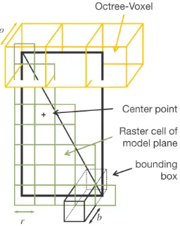
For the as-built as-planned comparison process, two different kind of grids are used. For checking visibility constraints, meaning to check which building elements are visible based on the rays from the cameras to the reconstructed points, a voxel grid with cells of sizeois created. This grid is generated for the whole construc-tion site area. Addiconstruc-tionally every triangle-plane of the as-planned model is split into quadratic raster cells of size r. Both grids are depicted in Figure 1 together with a building element’s sur-face which is split into two triangles. The voxel grid is shown in orange, the raster cells are shown in green. The voxel grid is typically not aligned orthogonally to the model planes (as it is for simplicity here in the figure), but to the coordinate system axes of the model. The center point shown in the figure is used as a ref-erence coordinate for the raster cells. The bounding box around each raster cell is used to extract points in front and behind the model plane with the maximum distanceb.
Figure 1. Main components for the as-built as-planned compar-ison. The black rectangle represents a surface of a building ele-ment split into two triangles. The orange octree cells are used for visibility checks. The green raster cells split each triangle into smaller elements. For each raster cell a measure is calculated based on the points extracted by the bounding box.
2.2 Visibility checks
built upon element 4. A concept for the identification and the use of this information is presented in (Braun et al., 2015) where a precedence relationship graph is used to represent technological dependencies.
Figure 2. General principle of the visibility checks visualized based on a cross-section through the voxel grid. As example, the rays from one camera to the 3D points reconstructed by this camera are depicted. Voxel cells are labeled asoccupied,freeor
unknownbased on this rays.
For the implementation of the visibility constraints the octomap library is used (Hornung et al., 2013). Every voxel cellnvoxis updated based on a probabilistic approach for repeated observa-tion of the same grid cell. Repeated measurementsziare caused by rays of multiple images observing the same object. The inte-gration of the measurements is performed using occupancy grid mapping as introduced by (Moravec and Elfes, 1985). As shown by (Hornung et al., 2013) this can be written in log-odd notation as in Equation 1 if a uniform prior probability and a clamping update policy is used:
L(n|z1:i) =
max(min(L(n|z1:i−1) +L(n|zi), lmax), lmin) (1)
with
L(n) =log
P(n) 1−P(n)
(2)
lminandlmax(as log-odds) denote the lower and upper bounds (clamping thresholds) of the log odd-valuesL(n).
Using this calculation, a probabilityPvis, whose value ranges fromlmintolmax(as probabilities), is determined for every voxel cell. A labelfree,occupiedorunknowncan be inferred from this value. The labelunknownis a clear assignment, in this case no value is present. The labelsfreeandoccupiedare assigned based on the thresholdstf reeandtoccon the probabilityPvis(nvox)of the respective voxel cell. Figure 3 visualizes how the information from the labeled voxel grid is used. At the position of each center point the label from the voxel grid is assigned to the respective raster cell. As shown before, the size of the voxel cellsois set larger than the size of the raster cellsrsince the main objective for the visibility check is to identify objects which are clearly not existent (i.e., free cells) or not visible (i.e., unknown cells). If a large cell isfreeorunknownthis has to be also valid for all smaller cells inside. Another constraint is, that reducing the voxel size is limited because of computational reasons. It is assumed that the large cell size will lead to discretization errors. Thus it is obvious that occupied cells cannot be used to verify building elements, since the existence of an object close to the expected plane (if within the same voxel cell) will also lead to marking a
raster cell as occupied. As a consequence, an additional measure is introduced in the next section.
Figure 3. Usage of the voxel grid introduced in Figure 1. After the visibility check one of three states is assigned to each voxel cell. Subsequently each raster cell of the triangle receives the state of the voxel grid cell at the position of its center point.
2.3 Point-Model-Distance
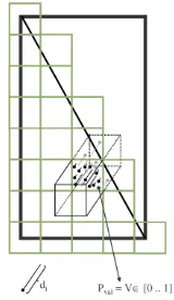
To decide if a building surface element can be verified, the sur-rounding points of a raster cell, as shown in Figure 4, are used. For every raster cellnrasthe valuePval ∈ [0..1]is calculated based on the points before and behind the model surface, which expresses the belief that this part of the surface is verified by the points. To calculate this value three criteria are used:
– Mean valueµdof the absolute values of the orthogonal dis-tancesdibetween the points and the triangle surface.
– The angleαbetween the normal of the model surface and the normal of a plane fitted to the extracted points.
– Standard deviation of the absolute values of the distancesdi.
Figure 4. Usage of the raster cells introduced in Figure 1 for calculation of the measurePval. The measure is based on the orthogonal distancediof the points within the bounding box.
the points and the co-registration accuracy. For the evaluation of the angle deviation, the tolerance thresholdtolα[◦] has to be introduced to define the maximum allowable deviation that can contribute to the verification of the raster cell. Deviations larger thantolα,max receive the minimum valuelmin as probability. The parameterslminandlmax are the clamping thresholds (as used in Equation 1) and also define the maximum and minimum probability for all three cases.
Equation 3 models the weighting based on the mean valueµd. A small mean value is necessary to confirm the surface. If the mean value is smaller than half of the thresholdtol, it contributes with the maximum probability. From this position the probability de-creases linearly to the minimum probability value at the position of 1.5tol:
P(nras|z1) =
P(µd) =
lmax if:µd<0.5·tol
p1(µd) if:0.5·tol < µd<1.5·tol lmin if:µd>1.5·tol
(3)
with
p1(µd) =
lmin−lmax
tol ·µd+ 1.5·lmax−0.5·lmin (4)
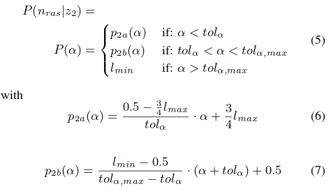
Equation 5 models the weighting considering the angle deviation α. Since only planar surfaces are examined if a triangle mesh is used, a planar object with the same orientation is necessary to confirm the triangle. Consequentlyαonly contributes to con-firm the object if its value is smaller thantolα. The probability decreases linearly from 0 degree totolα, starting with the proba-bility 3/4lmaxfor no deviation (cf. Equation 6).
P(nras|z2) =
P(α) =
p2a(α) if:α < tolα
p2b(α) if:tolα< α < tolα,max lmin if:α > tolα,max
(5)
with
p2a(α) =
0.5−3 4lmax
tolα
·α+3
4lmax (6)
p2b(α) =
lmin−0.5 tolα,max−tolα
·(α+tolα) + 0.5 (7)
Finally, Equation 8 models the weighting considering the stan-dard deviation of the distances. Since a small stanstan-dard deviation does not proof the existence of the correct object a small stan-dard deviation leads to a neutral weighting (= 0.5), but for large standard deviations probabilities smaller than 0.5 are introduced.
P(nras|z3) =
P(σd) =
0.5 if:σd< tol
p3(σd) if:tol < σd<2·tol lmin if:σd>2·tol
(8)
with
p3(σd) =
lmin−0.5
tol ·σd+ 1−lmin (9)
3. EXPERIMENT
3.1 Data
For the evaluation of the approach data sets of two different time steps (15 May (1) and 27 June 2013 (2)) are used. The images are acquired using hand-held terrestrial cameras. The resulting point clouds are shown in Figure 5 and 6. They are both compared to the as-planned model for 27 June (shown in Figure 7). The model consists of 11894 triangles. Using a raster size ofr= 10 cm this leads to a total number of 835037 raster cells for 9689 triangles. The remaining 2205 triangles are smaller than the raster size and not further considered.
Figure 5. Point cloud for time step 1 on 15 May.
Figure 6. Point cloud for time step 2 on 27 June.
Figure 7. As-planned model in triangle representation for time step 2 on 27 June.
3.2 As-built as-planned comparison
For the as-built as-planned comparison an octree grid size ofo= 15 cm and a raster cell size ofr= 10 cm is selected.
cells having a probabilityPvissmaller thantf ree = 0.2are la-beled asfreeand cells having a probability larger thantocc= 0.8 are labeled asoccupied. These thresholds are selected to ensure reliable labels what is motivated in the results section (3.3). As a result of the visibility check, building elements are extracted which can be clearly classified asnot builtor asnot visibleand which can be classified aspotentially built. A building element is regarded asnot built if 90% of its raster cells are labeled as
free. A building element is regarded asnot visibleif 90% of its raster cells are labeled asunknown. Finally a building element is regarded aspotentially builtif at least 33% of the raster cells are labeled asoccupied. The elements classified aspotentially builtare further analyzed using the approach described in Section 2.3 to calculate the valuePvalfor every raster cell. Therefore, a bounding box size ofb= 5 cm is used. The tolerancetolhas to be smaller than the distance for the extraction of the points and is set to 2.5 cm. This value is inferred from the typical depth accuracy which can be achieved with the selected acquisition geometry. A loose threshold for the angle deviationtolα= 45◦is selected due to the fact that a plane is fitted to a small patch of the point cloud (10x10x10 cm). In combination with noisy points this may result in large deviations even if the plane exists. The minimum and maximum values for the probability are selected closely to zero and one withlmin= 0.01andlmax= 0.99(consider that these two values can be chosen differently for the visibility checks and the calculation ofPval).
A raster cell is accepted as verified ifPval>0.5. Then the verifi-cation rateVR(Equation 10) can be calculated, which is the ratio of the verified raster cells to all raster cells of one triangle. Raster cells having the labelunknownare excluded from that calcula-tion, so that only the visible elements of the triangles are taken into account.
V R=
P
nras,verif ied
P
nras−Pnras,unknown
(10)
Finally, a threshold can be applied to decide if a building element triangle is verified as being built, or the verification rate can be assigned to every triangle. In the results shown in the next sec-tion every triangle is given the statebuiltif the verification rate is larger than 50%. A summary of all states and their dependencies is given in Table 1.
Table 1. Dependencies of states.
3.3 Results
In Figures 8 and 9 the results for the visibility checks are shown. All triangles marked in blue are labeled asnot visible, the red tri-angles are labeled asnot builtand the green triangles are labeled aspotentially built. In Table 2, the number of triangles for each label are given. Triangles not classified as one of the states are in the group rest and are not shown in the figures. The number of triangles in this group is relatively large because the thresholds are strict for the labelsunknownandfree. The strict threshold is used to ensure a reliable labeling for these two states. Since the threshold on the percentage of occupied cells for the label poten-tially builtis rather loose, the group rest is composed of triangles
which are built butnot visibleand which arenot built. In the re-sults for time step 1 there is a large area marked asfreesince the as-planned state for the second time step is used. To be able to mark areas asfree, points have to be reconstructed behind the pre-dicted planes, otherwise no rays pass through these planes. This explains that the upper part in Figure 8 is labeled asunknown. In both cases the most triangles are labeled asunknown, what can mainly be ascribed to three reasons:
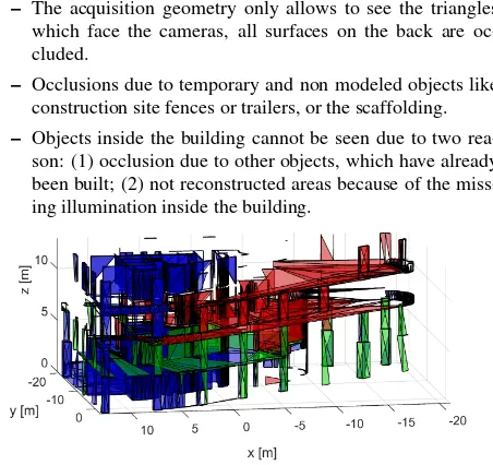
– The acquisition geometry only allows to see the triangles which face the cameras, all surfaces on the back are oc-cluded.
– Occlusions due to temporary and non modeled objects like construction site fences or trailers, or the scaffolding.
– Objects inside the building cannot be seen due to two rea-son: (1) occlusion due to other objects, which have already been built; (2) not reconstructed areas because of the miss-ing illumination inside the buildmiss-ing.
Figure 8. Result of the visibility checks for the point cloud of time step 1 (Figure 5). Green triangles are labeled aspotentially built, blue triangles are labeled asnot visibleand red triangles are labeled asnot built.
Figure 9. Result of the visibility checks for the point cloud of time step 2 (Figure 6). Green triangles are labeled aspotentially built, blue triangles are labeled asunknownand red triangles are labeled asnot built.
15 May 27 June
not built (red) 1281 13.2% 157 1.6% not visible (blue) 3360 34.7% 6742 69.6% pot. built (green) 871 9.0% 493 5.1%
rest 4177 43.1% 2297 23.7%
Table 2. Numerical results for the visibility checks: the number of triangles for each class are given
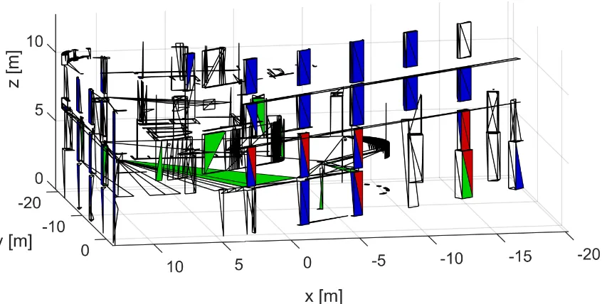
Figure 10. Final result showing the confirmed triangles for both time steps. Triangles labeled aspotentially builtbut have not been confirmed are uncolored. The green triangles are confirmed by the point cloud of time step 1, blue triangles are confirmed by the point cloud of time step 2 and red triangles are confirmed in both of the time steps.
15 May, the blue triangles indicate the elements confirmed by the point cloud from 27 June and the red triangles indicate the ele-ments confirmed by both point clouds. On 15 May, 109 triangles (12.5% ofpotentially built) and on 27 June, 99 triangles (20% of
potentially built) are confirmed. All verifications are correct ex-cept from 2 triangles on each time step. In these cases, building elements are confirmed when a formwork is installed. However, a lot of built elements are not recognized, partly at areas with limited reconstruction accuracy, but mainly because of the insuf-ficient coverage with points. Other elements are correctly marked asnot builteven if they seem to be built. This can be ascribed to the modeling. At the ceiling slabs the faces looking towards the outside of the building are modeled with an additional insulation in the BIM, despite the fact that it has been mounted later. The structural elements are not modeled as a seperate part. Since the insulation is in front of the concrete slabs these elements are cor-rectly not confirmed as being built. For the second time step these elements are mainly classified to the group rest. The reason is that points of temporary objects like the scaffolding and the formwork exist inside the area of the coming insulation, so that these ele-ments cannot unambiguously be labeled asfreeorunknown. There is no evaluation based on the number of triangles for two reasons: On the one hand not all triangles can be marked unam-biguously asbuiltornot builtfor ground truth. On the other hand the different size and amount of triangles for different building elements would lead to no representative results.
4. DISCUSSION AND OUTLOOK
In this paper an approach is introduced for the validation of build-ing parts of a triangulated 4D model. It is shown that the triangles can be correctly marked asbuiltornot built. The statements are all correct with only a few exceptions for the case when a form-work is installed. This shows the feasibility of making robust statements about the state of single building parts. The drawback is that there are a lot of triangles (around 75% in time step 1 and more than 90 % in time step 2) where no statement can be made. This is mainly due to the fact that it is impossible to make these parts visible in the acquired data. Moreover, there are some parts where the data acquisition is insufficient in terms of coverage or
accuracy.
This is still work in progress and various improvements can be made towards an operational applicability. Some enhancements can be made by optimizing the data acquisition. The framework for the validation of the raster cells can be easily extended with additional criteria, like the color of the points. Furthermore, it is important to introduce knowledge about the construction pro-cesses and technological dependencies modeled in the BIM to make statements about building parts which are not or only partly visible. For this further processing it has to be ensured that the labels based on the as-built data are correct.
A problem which has to be further investigated is, how errors in the process can be ascribed to their respective source. It has to be distinguished if deviations between point cloud and model are due to the orientation accuracy of the images, inaccuracies in the reconstruction process, errors in the co-registration, erroneous modeling of the building, errors in the building construction, or due to disturbing or temporary objects.
The usage of triangles makes the processing easier than using more complex geometric shapes since every object can be decom-posed into the same simple basic geometry. Also curved parts can be handled this way. Disadvantages are that there are partly very small triangles, some of them smaller than the raster size used for computation of the labels, and that single surfaces (e.g. rectan-gles) are split into several parts which are treated individually. In terms of coverage of the construction site other data acqui-sition techniques will be tested in future. On the one hand the acquisition using an UAV, on the other hand cameras mounted at the boom of a crane. In both cases data can be acquired for monitoring even if the construction sites are covered.
ACKNOWLEDGEMENTS
We also would like to thank Konrad Eder for his support during the data acquisition.
REFERENCES
Bosch´e, F., 2010. Automated recognition of 3d cad model objects in laser scans and calculation of as-built dimensions for dimen-sional compliance control in construction. Advanced Engineering Informatics 24(1), pp. 107–118.
Bosch´e, F. and Haas, C. T., 2008. Automated retrieval of 3d cad model objects in construction range images. Automation in Construction 17(4), pp. 499–512.
Braun, A., Borrmann, A., Tuttas, S. and Stilla, U., 2014. To-wards automated construction progress monitoring using bim-based point cloud processing. In: A. Mahdavi, B. Martens and R. Scherer (eds), ECPPM 2014, CRC Press, pp. 101–107.
Braun, A., Borrmann, A., Tuttas, S. and Stilla, U., 2015. A con-cept for automated construction progress monitoring using bim-based geometric constraints and photogrammetric point clouds. Journal of Information Technology in Construction 20, pp. 68 – 79.
Brilakis, I., Fathi, H. and Rashidi, A., 2011. Progressive 3d re-construction of infrastructure with videogrammetry. Automation in Construction 20(7), pp. 884–895.
Fathi, H. and Brilakis, I., 2011. Automated sparse 3d point cloud generation of infrastructure using its distinctive visual features. Advanced Engineering Informatics 25(4), pp. 760–770.
Golparvar-Fard, M., Bohn, J., Teizer, J., Savarese, S. and Pe?a-Mora, F., 2011a. Evaluation of image-based modeling and laser scanning accuracy for emerging automated performance moni-toring techniques. Automation in Construction 20(8), pp. 1143– 1155.
Golparvar-Fard, M., Pe˜na Mora, F. and Savarese, S., 2012. Au-tomated progress monitoring using unordered daily construction photographs and ifc-based building information models. Journal of Computing in Civil Engineering.
Golparvar-Fard, M., Pena-Mora, F. and Savarese, S., 2011b. Monitoring changes of 3d building elements from unordered photo collections. In: Computer Vision Workshops (ICCV Work-shops), 2011 IEEE International Conference on, pp. 249–256.
Hornung, A., Wurm, K., Bennewitz, M., Stachniss, C. and Bur-gard, W., 2013. Octomap: an efficient probabilistic 3d map-ping framework based on octrees. Autonomous Robots 34(3), pp. 189–206.
Ibrahim, Y. M., Lukins, T. C., Zhang, X., Trucco, E. and Kaka, A. P., 2009. Towards automated progress assessment of work-package components in construction projects using computer vi-sion. Advanced Engineering Informatics 23(1), pp. 93–103.
Kim, C., Kim, B. and Kim, H., 2013a. 4d cad model updating using image processing-based construction progress monitoring. Automation in Construction 35, pp. 44–52.
Kim, C., Son, H. and Kim, C., 2013b. Automated construction progress measurement using a 4d building information model and 3d data. Automation in Construction 31, pp. 75–82.
Moravec, H. P. and Elfes, A., 1985. High resolution maps from wide angle sonar. In: Robotics and Automation. Proceedings. 1985 IEEE International Conference on, Vol. 2, pp. 116–121.
Rankohi, S. and Waugh, L., 2014. Image-based modeling ap-proaches for projects status comparison. In: CSCE 2014 General Conference.
Rashidi, A., Brilakis, I. and Vela, P., 2014. Generating absolute-scale point cloud data of built infrastructure scenes using a monocular camera setting. Journal of Computing in Civil En-gineering pp. 04014089–1 – 04014089–12.
Son, H. and Kim, C., 2010. 3d structural component recognition and modeling method using color and 3d data for construction progress monitoring. Automation in Construction 19(7), pp. 844– 854.
Turkan, Y., Bosch´e, F., Haas, C. and Haas, R., 2013. Toward automated earned value tracking using 3d imaging tools. Journal of Construction Engineering and Management 139(4), pp. 423– 433.
Turkan, Y., Bosch´e, F., Haas, C. T. and Haas, R., 2012. Auto-mated progress tracking using 4d schedule and 3d sensing tech-nologies. Automation in Construction 22, pp. 414–421.
Turkan, Y., Bosch´e, F., Haas, C. T. and Haas, R., 2014. Track-ing of secondary and temporary objects in structural concrete work. Construction Innovation: Information, Process, Manage-ment 14(2), pp. 145–167.
Tuttas, S., Braun, A., Borrmann, A. and Stilla, U., 2014a. Com-parison of photogrammetric point clouds with bim building ele-ments for construction progress monitoring. In: Int. Arch. Pho-togramm. Remote Sens. Spatial Inf. Sci., Vol. XL-3, Copernicus Publications, pp. 341–345. ISPRS Archives.
Tuttas, S., Braun, A., Borrmann, A. and Stilla, U., 2014b. Konzept zur automatischen baufortschrittskontrolle durch in-tegration eines building information models und photogram-metrisch erzeugten punktwolken. In: E. Seyfert, E. G?lch, C. Heipke, J. Schiewe and M. Sester (eds), Gemeinsame Tagung 2014 der DGfK, der DGPF, der GfGI und des GiN, pp. 363–372.