Identifying sources and sinks of scalars in a corn canopy
with inverse Lagrangian dispersion analysis
I. Heat
O.T. Denmead
a,∗, L.A. Harper
b, R.R. Sharpe
baCSIRO Land and Water, F.C. Pye Laboratory, GPO Box 1666, Canberra, ACT 2601, Australia
bSouthern Piedmont Conservation Research Center, USDA-ARS, 1420 Experiment Station Road, Watkinsville, GA 30677, USA
Abstract
Sources and sinks of heat in the canopy of a dense corn crop (LAI∼5) were inferred through an inverse Lagrangian dispersion analysis. Input data were the profiles of air temperature and turbulence above and within the canopy. The analysis was verified in part by comparing its predictions of the net exchanges of sensible heat between canopy and air with direct measurements of the sensible heat flux above the crop made by eddy correlation.
Almost all the heat exchange occurred in the top half of the canopy, which was a strong heat source. The bottom half was a weak sink, virtually neutral in the overall heat exchange. The net exchanges of heat predicted by the analysis were, on average, 21% higher than the eddy correlation heat fluxes, but exhibited identical time trends. It is concluded that the inverse Lagrangian technique leads to robust and qualitatively correct predictions of the heat flux and that the analysis scheme employed offers a relatively simple means for calculating scalar fluxes in plant canopies. © 2000 Elsevier Science B.V. All rights reserved.
Keywords: Turbulence; Diffusion; Canopy transport; Canopy modelling; Energy exchange; Heat flux
1. Introduction
Many investigations of the exchange of scalars such as heat, water vapour and trace gases, between plant communities and the atmosphere require in-formation on the distribution of sources and sinks within the canopy space. Evapotranspiration and CO2
assimilation are good examples of relevant exchange processes. Understanding each requires knowledge of the separate contributions to the net exchange by plants and soil. Seminal contributions in these fields include analyses of the relative importance of soil and
∗Corresponding author. Fax:+61-2-6246-5560.
E-mail address: [email protected] (O.T. Denmead)
plant evaporation in the overall water loss from crops by John Monteith and his mentor, Howard Penman (Penman and Long, 1960; Monteith, 1965), Monteith’s investigations of the role of soil respiration and plant assimilation in the CO2exchange of crops (Monteith,
1962; Monteith et al., 1964) and of course, Monteith’s introduction of the concept of crop and canopy resis-tances to examine gas exchange in plant communities (Monteith, 1963).
Emission of ammonia following application of ni-trogen fertiliser is another instance where informa-tion on canopy sources and sinks is necessary. In this case, NH3 can be emitted from the soil and
ab-sorbed or emitted from the foliage. Formulation of effective emission control measures will depend on
the relative importance of the soil and plant sources (or sinks). In a companion paper, we examine source and sink distributions of NH3within the canopy of a
corn crop irrigated with dairy effluent (Harper et al., 2000).
Early attempts at identifying sources and sinks of scalars in plant canopies used gradient-diffusion ap-proaches in which the scalar was assumed to be trans-ported by turbulent diffusion along its concentration gradient from regions of high to low concentration. Formally, such transport is described by
FS(z)= −K(z)
∂C
∂z (1)
where FS represents the flux of the scalar at height z, K is a height-dependent eddy diffusivity and C is the scalar concentration. It has been demonstrated, however, that such a description can give quite misleading pictures of transport within the canopy space (Denmead and Bradley, 1985, 1987). Appar-ent counter-gradiAppar-ent flows occur commonly in plant canopies, i.e. the transport is in an opposite direction to that indicated by the sign of the concentration gradient. Alternative descriptions have been devel-oped in consequence. These include higher-order closure models (Wilson and Shaw, 1977; Finnigan and Raupach, 1987), large-eddy simulation (Shaw and Schumann, 1992), wavelet analysis (Collineau and Brunet, 1993) and Lagrangian dispersion models (Raupach, 1989a,b,c; Raupach et al., 1992; Den-mead, 1995). The first three approaches require rapid measurement of instantaneous scalar concen-trations. The inverse Lagrangian dispersion model developed by Raupach (1989b), however, permits the identification of scalar sources and sinks in the canopy space from measurements of mean concen-tration profiles which are usually much easier to obtain.
The present paper validates inverse Lagrangian dispersion analysis in a corn canopy by examining the transport of heat. The net exchanges of sensible heat between canopy and atmosphere predicted by the analysis are compared with direct measurements made by eddy correlation. A companion paper by Harper et al. (2000) applies the model to an exam-ination of NH3 exchange between soil, plants and
atmosphere.
2. The inverse Lagrangian dispersion model
The model is based on theoretical developments by Raupach (1989a,b,c). Here, we give only a brief qual-itative description of its theoretical basis.
The model considers dispersion in regions near to and far from canopy source elements (the foliage and the ground). Scalar concentrations within and above the canopy result from contributions from the near field and the far field
C(z)=Cn(z)+Cf(z) (2)
where the subscripts n and f refer to the near and far fields, respectively. In the near field which extends about one canopy height downwind of a particular source, dispersion is dominated by the local coherence of eddy motions. In the far field, dispersion is dom-inated by the randomness of the turbulence and dis-persion there can be described by gradient-diffusion following Eq. (1), viz.
F (z)= −Kf(z)
∂Cf
∂z (3)
The near field concentration Cn is obtained from
knowledge of the source strength S and the turbu-lence. The latter is characterised byσw, the standard deviation of the vertical wind speed w, and TL, the
Lagrangian time scale for vertical velocity, which is a measure of the average coherence time of eddies. Cal-culation of Cnfollows the model of Raupach (1989a).
In practical applications, the profile ofσw above and within the canopy is a model input based on ensem-ble averaged measurements for that canopy. TLis
ob-tained empirically from the canopy height h and the friction velocity u∗above the canopy, both of which
are also model inputs.
The far field concentration Cfis obtained by solving
Eq. (3) with
Kf(z)=σw2(z)TL(z) (4)
Through these equations, Raupach (1989b) relates concentrations at any level i (i=1–n) to the source strengths at levels j within the canopy (j=1–m) using a dispersion matrix D with coefficients Dij.
Ci−CR=
X
j
where CR is the concentration at a reference level
above the canopy, m represents the number of discrete layers in the canopy for which solutions are required, each layer having strength Sjand depth1zj. Raupach (1989a,b) gives procedures for calculating the coeffi-cients Dij from u∗,σw and TL.
Eq. (5) is the solution to the forward Lagrangian dispersion problem, i.e. that of predicting the concen-tration profiles generated by a given source–sink dis-tribution. Raupach (1989b) shows how to extend the dispersion analysis to the inverse problem: determin-ing source strengths from mean concentration profiles. Once the input data are assembled, the analysis can be performed on a personal computer in a matter of seconds. One practical requirement of the procedure is that the number of source layers be less than the number of heights for which concentration data are available. We note that the net flux of the scalar from the canopy is given by
FS(h)=
X
j
Sj1zj (6)
Examples of the use of inverse Lagrangian dispersion analysis are given by Raupach (1989b) for studying the dispersion of heat from an elevated plane source in a model canopy in a wind-tunnel, by Denmead and Raupach (1993) and Denmead (1995, 1996) for de-termining source- and sink-strengths for heat, water vapour and CO2in crops of wheat and sugar cane and
by Harper et al. (2000) for investigating pathways of NH3loss within a corn canopy.
3. Materials and methods
3.1. Crop
The research was conducted in a crop of irrigated corn (Zea mays L.) grown for silage at Montezuma, GA, USA. The study was conducted during a period of 20 days after anthesis, from 13 June to 2 July 1993. The corn was planted at a density of 77,000 plants ha−1with starter fertilizer nitrogen (N) applied at 27 kg N ha−1. During the growing season, further N was supplied by regular sprinkler application of dairy waste effluent. At the commencement of the study, the crop had a leaf area index (LAI) of 4.95 and was 2.7 m
high. At the end of the study, the LAI was 5.3 and crop height was 3.3 m. LAI was determined by measuring the areas of all leaves on each of 10 plants selected randomly, and dividing that area by the ground area occupied by the plants. The height interval occupied by each leaf was also recorded in order to calculate the LAI in each of four canopy layers employed for the inverse Lagrangian analysis (Section 3.2.1).
3.2. Micrometeorological
As indicated above, the net heat fluxes from the canopy calculated by the inverse Lagrangian analysis were compared with heat fluxes above the crop mea-sured by eddy correlation. Input data for the analysis were temperature profiles within the canopy and above it.
3.2.1. Temperature
In this study, source densities for heat were calcu-lated for four layers of equal depth in the canopy us-ing measurements of air temperature at eight levels, viz. 0.45, 0.9, 1.35, 1.8, 2.25, 2.7, 3.3 and 4.3 m above the ground on 13 June and 0.55, 1.10, 1.65, 2.2, 2.75, 3.3, 3.9 and 4.9 m for observations made on 29 June, 30 June, 1 July, and 2 July. The sixth measurement in each list was at h, while the seventh and eighth were above the canopy. The thermometers were aspi-rated, double radiation-shielded, three-junction, cop-per/constantan thermocouples. The fans were of the squirrel-cage type and were designed to give an air-speed of 3 m s−1over the thermocouples. The sensors
were cross-calibrated with measurements at the same point and in profile mode. Electronic noise was about 0.01◦C.
3.2.2. Turbulence measurements
σw and u∗ were measured 5 m above the ground
with a Dobbie three-dimensional sonic anemometer with a 0.1 m path length (Coppin and Taylor, 1983).
u∗= −w′u′ 1/2
(7)
where u is horizontal velocity, the primes denote de-viations from the means and the overbar represents a time average.
canopy) using published data of Wilson et al. (1982). Their data for corn indicate that
z
h ≥1, LAI=0, σw =σw(h),
z
h<1, 0<LAI≤3,
σw=(1−0.283LAI)σw(h), (8)
z
h <1, LAI>3, σw =0.15σw(h)
The correlation betweenσw/σw(h) and LAI in the data of Wilson et al. (1982) is very strong, with r2=0.996. Theσw/σw(h) relationship for LAI>3 is an extrapo-lation of those data. In order to perform the inverse Lagrangian analysis, it was necessary to express Eq. (8) in terms of z rather than LAI. This was accom-plished by fitting a third-order polynomial to mea-surements of the distribution of LAI with z, for which r2=0.996 also. The final form of the dependence of
σw on z used in the analysis is shown in Fig. 1.
3.2.3. Eddy correlation measurements
The sonic anemometer measurements were com-bined with measurements of temperature T at 5 m made with a fast-response, fine-wire, resistance ther-mometer in order to obtain the sensible heat flux H.
Fig. 1. Assumed profile of normalisedσwabove and within the
corn canopy following Wilson et al. (1982). h denotes canopy height.
H=ρcpw′T′ (9)
whereρis air density and cpis the specific heat of air
at constant pressure.
A cross comparison between the mean temperatures indicated by the resistance thermometer at 5 m and the thermocouple thermometer at 4.9 m showed a differ-ence of 6% between the two, which was fed into the calculation of the eddy correlation H. That calculation also applied corrections of approximately 10% to the apparent H to account for different averaging paths for the wind and temperature sensors and for sensor separation (Moore, 1986).
3.2.4. Sampling periods
The micrometeorological data were collected in successive 0.5 h runs. Data collection periods varied from 4.5 h on 29 June to 9.5 h on 1 July.
4. Results and discussion
4.1. Heat fluxes from inverse Lagrangian dispersion analysis
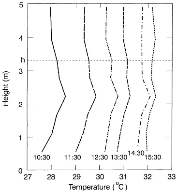
4.1.1. Temperature profiles
Fig. 2 shows representative temperature profiles for one day in the study, 2 July. A notable feature in all
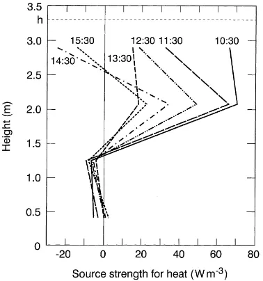
Fig. 3. Source strengths for sensible heat calculated by the inverse Lagrangian analysis for the temperature profiles in Fig. 2.
profiles is the existence of a ‘hot spot’ at about 2/3 canopy height during the daytime, which indicates a region of strong heat production there. The same fea-ture was present during high radiation periods on all days during the study.
4.1.2. Source–sink distributions within the canopy Fig. 3 shows the distribution of heat sources in the canopy, calculated by the inverse Lagrangian disper-sion analysis, for the temperature profiles in Fig. 2. It is evident that the canopy was a net heat source for most of the day, with strong heat production around the ‘hot spot’. Foliage in the top layer changed from a heat source in the morning to a heat sink in the after-noon, while the bottom foliage and the soil constituted weak heat sinks for most of the day. Very much the same source distribution was observed on each day of measurement, as can be seen in Fig. 4 which shows the average cumulative heat flux through the canopy for each day.
4.2. Comparison with conventional micrometeoro-logical measurements
While it was not possible to test the predictions of the analysis layer by layer, it was possible to
com-Fig. 4. Average cumulative heat fluxes in the canopy calculated by the inverse Lagrangian analysis for 5 days of measurement.
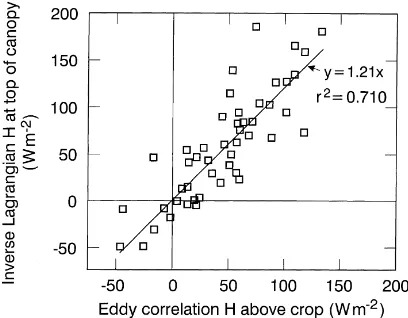
pare its predictions of the net exchanges of heat for the canopy, i.e. the cumulative heat flux at the canopy top, with the independent eddy correlation measure-ments of H at 5 m. Fig. 5 shows both heat fluxes on 3 days: the example day of 2 July and two previous days, 30 June and 1 July. The time courses of the in-verse Lagrangian fluxes closely followed those of the eddy correlation measurements, but the magnitude of the former was often somewhat higher. Fig. 6 com-pares all the inverse Lagrangian estimates of the net canopy heat flux with the directly-measured eddy cor-relation fluxes. As noted already, the qualitative agree-ment between the two was good (r2=0.710), but the inverse Lagrangian fluxes were 21% higher.
Fig. 5. Net exchanges of heat between canopy and air inferred by inverse Lagrangian analysis and measured by eddy correlation.
inverse Lagrangian dispersion analyses. In most of the analyses in the present study, conditions were mod-erately unstable. From the work of Leuning (2000), this would have resulted in negligibly small correc-tions that, in any case, would have made the inverse Lagrangian predictions of the heat flux marginally higher. It is possible that the discrepancy resulted from small, systematic errors in the temperature measurements. Achieving a perfect match between eight thermometers is very difficult. As illustrated in Fig. 2, the temperature variation over the whole pro-file was usually less than 1◦C, so that small errors in
thermometer readings or calibrations could produce relatively large errors in the overall estimate of the heat flux. Whatever the cause, it is still the case that
Fig. 6. Comparison of inverse Lagrangian and eddy correlation heat fluxes for all available data.
the inverse Lagrangian technique provided a robust and qualitatively correct estimate of the net heat flux from the canopy, in reasonably close agreement with independent measurements. This gives confidence in the analysis of sources and sinks of ammonia in the canopy presented by Harper et al. (2000), which relies on the same general approach.
5. Conclusions
The inverse Lagrangian dispersion analysis outlined here provided stable, qualitatively correct estimates of the net exchange of heat between canopy and atmo-sphere. The estimates were 21% higher than direct measurements of heat flux by eddy correlation, per-haps due to small systematic measurement or calibra-tion errors in the thermometer array used to define the within-canopy temperature profiles. Both heat flux measurements showed the same diurnal trends and the correlation coefficient between them was 0.84.
Almost all the heat exchange between foliage and air occurred in the top half of the dense corn canopy which, overall, constituted a strong heat source. The bottom half was a very weak heat sink, virtually neu-tral in terms of the overall heat exchange. We conclude that Raupach’s (1989b) analysis offers a robust and relatively simple measurement scheme for calculating scalar fluxes within plant canopies.
Acknowledgements
inverse Lagrangian analysis. The senior author wishes to thank USDA-ARS and the Southern Piedmont Conservation Research Center, Watkinsville, GA, for hosting him during the study.
References
Anderson, D.E., Verma, S.B., Rosenberg, N.J., 1984. Eddy correlation measurements of CO2, latent heat, and sensible heat fluxes over a crop surface. Boundary-Layer Meteorol. 29, 263–272.
Baldocchi, D., 1994. A comparative study of mass and energy exchange over a closed C3 (wheat) and an open C4 (corn) canopy. I. The partitioning of available energy into latent and sensible heat exchange. Agric. For. Meteorol. 67, 191–220. Collineau, S., Brunet, Y., 1993. Detection of coherent motions in
a forest canopy. I. Wavelet analysis. Boundary-Layer Meteorol. 65, 357–359.
Coppin, P., Taylor, K.J., 1983. A three component sonic anemo-meter/thermometer system for general micrometeorological research. Boundary-Layer Meteorol. 27, 27–42.
Denmead, O.T., 1995. Novel meteorological methods for measuring trace gas fluxes. Philos. Trans. R. Soc., London Ser. A 351, 383–396.
Denmead, O.T., 1996. Measuring and modelling soil evaporation in wheat crops. Phys. Chem. Earth 21, 97–100.
Denmead, O.T., Bradley, E.F., 1985. Flux-gradient relationships in a forest canopy. In: Hutchinson, B.A., Hicks, B.B. (Eds.), The Forest-Atmosphere Interaction. Reidel, Dordrecht, pp. 421–442.
Denmead, O.T., Bradley, E.F., 1987. On scalar transport in plant canopies. Irrig. Sci. 8, 131–149.
Denmead, O.T., Raupach, M.R., 1993. Methods for measuring atmospheric gas transport in agricultural and forest systems. In: Harper, L.A., Mosier, A.R., Duxbury, J.M., Rolston, D.E. (Eds.), Agricultural Ecosystem Effects on Trace Gases and Global Climate Change. American Society of Agronomy Special Publication 55, Madison, Wisconsin, pp. 19–43.
Finnigan, J.J., Raupach, M.R., 1987. Transfer processes in plant canopies in relation to stomatal characteristics. In: Zeigler, E.,
Farquhar, G.D., Cowan, I.R. (Eds.), Stomatal Function. Stanford University Press, pp. 385–429.
Harper, L.A., Denmead, O.T., Sharpe, R.R., 2000. Identifying sources and sinks of scalars in a corn canopy with inverse Lagrangian dispersion analysis. II. Ammonia. Agric. For. Meteorol. 104, 75–83.
Leuning, R., 2000. Atmospheric stability and estimation of source/sink distributions in plant canopies using Lagrangian dispersion analysis. Boundary-Layer Meteorol., in press. Monteith, J.L., 1962. Measurement and interpretation of carbon
dioxide fluxes in the field. Neth. J. Agric Sci. 10, 334–346. Monteith, J.L., 1963. Gas exchange in plant communities. In:
Evans, L.T. (Ed.), Environmental Control of Plant Growth. Academic Press, New York, pp. 95–112.
Monteith, J.L., 1965. Evaporation and environment. Symp. Soc. Exp. Biol. 19, 205–234.
Monteith, J.L., Szeicz, G., Yabuki, K., 1964. Crop photosynthesis and the flux of carbon dioxide below the canopy. J. Appl. Ecol. 1, 321–337.
Moore, C.J., 1986. Frequency response corrections for eddy correlation systems. Boundary-Layer Meteorol. 37, 17–35. Penman, H.L., Long, I.F., 1960. Weather in wheat: an essay in
micro-meteorology. Q.J.R. Meteorol. Soc. 86, 16–50. Raupach, M.R., 1989a. A practical Lagrangian method for relating
scalar concentrations to source distributions in vegetation canopies. Q.J.R. Meteorol. Soc. 113, 107–120.
Raupach, M.R., 1989b. Applying Lagrangian fluid mechanics to infer scalar source distributions from concentration profiles in plant canopies. Agric. For. Meteorol. 47, 85–108.
Raupach, M.R., 1989c. Stand overstorey processes. Philos. Trans. R. Soc., London Ser. B 324, 175–190.
Raupach, M.R., Denmead, O.T., Dunin, F.X., 1992. Challenges in linking atmospheric CO2 concentrations to fluxes at local and regional scales. Aust. J. Bot. 40, 697–716.
Shaw, R.H., Schumann, U., 1992. Large-eddy simulation of turbulent flow above and within a forest. Boundary-Layer Meteorol. 61, 47–64.
Wilson, J.D., Shaw, R.H., 1977. A higher order closure model for canopy flow. J. Appl. Meteorol. 16, 1197–1205.