Investment in site-specific crop management under uncertainty:
implications for nitrogen pollution control
and environmental policy
Madhu Khanna
∗, Murat Isik, Alex Winter-Nelson
Department of Agricultural and Consumer Economics, University of Illinois at Urbana-Champaign, 431 Mumford Hall, 1301 W. Gregory Dr., Urbana, IL 61801, USA
Abstract
This paper applies an option-pricing model to analyze the impact of uncertainty about output prices and expectations of declining fixed costs on the optimal timing of investment in site-specific crop management (SSCM). It also analyzes the extent to which the level of spatial variability in soil conditions can mitigate the value of waiting to invest in SSCM and influence the optimal timing of adoption and create a preference for custom hiring rather than owner purchase of equipment. Numerical simulations show that while the net present value (NPV) rule predicts that immediate adoption is profitable under most of the soil conditions considered here, recognition of the option value of investment indicates that it is preferable to delay investment in SSCM for at least 3 years unless average soil quality is high and the variability in soil quality and fertility is high. The use of the option value approach reveals that the value of waiting to invest in SSCM raises the cost-share subsidy rates required to induce immediate adoption above the levels indicated by the NPV rule. © 2000 Elsevier Science B.V. All rights reserved.
Keywords: Option value; Net present value; Nitrogen pollution control; Variable rate application; Price uncertainty; Timing of adoption; Cost-share subsidy
1. Introduction
The adverse effects of nutrient run-off from agri-cultural fields on water quality have drawn attention to the need to increase the efficiency with which nu-trients are used (Committee on Long Range Soil and Water Conservation, 1993). Conventional whole field management practices that apply inputs at a uniform rate across a field are a major source of inefficiency in input utilization whenever nutrient needs vary within the field. Conventional methods may achieve a
nutri-∗Corresponding author. Tel.:+1-217-333-5176; fax:+1-217-333-5502.
E-mail address: [email protected] (M. Khanna).
ent uptake as low as 30% of the applied nitrogen by plants (Legg and Meisinger, 1982).
Site-specific crop management (SSCM) provides an input efficiency enhancing alternative to con-ventional methods by acquiring information about spatial variability in soil conditions and using it to target input applications to match that variability. It relies on several interrelated components that include grid-based soil sampling and yield monitors linked to satellite-based global positioning systems (GPS) that provide geo-referenced information about the agro-nomic conditions and yields at various points in the field and identify the need for spatial variation in input application. Variable rate technologies (VRT) then use this information to vary input flow rates on-the-go,
using onboard computers, GPS and soil maps. Far-mers may adopt SSCM either by purchasing all com-ponents or by custom hiring VRT and purchasing the rest.
Most studies analyzing the profitability of SSCM have relied on cost and yield data generated from on-field experiments (reviewed in Swinton and Lowenberg-DeBoer, 1998). Differences in experi-mental designs and agronomic conditions as well as in the types of variable and fixed costs that these stud-ies consider makes it difficult to compare their results and to arrive at generalizable conclusions valid for other field conditions. Some studies use simulation models to examine the impact of SSCM on farm pro-fitability (Schnitkey et al., 1996; Babcock and Pautsch, 1998) and on the environment (Watkins et al., 1998; Thrikawala et al., 1999). These studies show that SSCM has a potential to increase crop yields, reduce input-use and reduce input residues in the soil. These studies, however, implicitly assume that either future costs and revenues are certain or the investment is re-versible and expenditures can be recovered if market conditions turn out to be worse than anticipated.
Despite their potential for providing both economic and environmental benefits, recent surveys of farmers show low rates of adoption of SSCM. Only 4% of farmers had adopted VRT and 6% had adopted yield monitors in the US by 1996 (Daberkow and McBride, 1998). The corresponding figures for the Midwest were 12 and 10% (Khanna et al., 1999). Most of these adopters were custom hiring at least some of the services of site-specific technologies rather than purchasing them outright. Uncertainty about payback and high costs of adoption ranked as one of the two most important reasons for non-adoption by a ma-jority of the farmers surveyed. Sixty-one percent of the farmers indicated that they would be willing to adopt SSCM if a cost-share subsidy of up to 50% were offered. The survey also showed that farmers are delaying investment in SSCM and adoption rates are expected to increase almost fourfold in the next 5 years.
These observations are consistent with research that emphasizes the importance of analyzing the impact of sunk investment costs and uncertainty in returns on the timing of the decision to adopt a technology (Dixit and Pindyck, 1994). Historical data on corn prices show that price fluctuations were as large as 35–50%
during the 1970s and 1980s.1 With the exception of the 1970s, market prices have been generally below the target price of corn, necessitating deficiency pay-ments to farmers. The FAIR Act (1996) by dismantling government supply controls and price stabilizing pro-grams, is expected to increase variability in corn prices in the future (Ray et al., 1998). Corn price movements since 1996 provide some evidence of this variability. Corn prices rose to a 10-year high in 1996 and fell by 40% to a 5-year low in 1998.
Since site-specific technologies are still in their in-fancy and undergoing rapid improvements, the result-ing technological obsolescence of existresult-ing equipment makes it unlikely that farmers that have invested in SSCM could recover their sunk costs if the investment were to be liquidated. Additionally, prices of equip-ment for site-specific technologies can be expected to fall as growing demand leads to economies of scale in their manufacture. For example, the cost of Ag Leader yield monitors and GPS receivers has fallen by over 10% between 1997 and 1999. If adjusted for quality improvements, this decline in equipment costs would be even larger. Given uncertainty in prices and the ir-reversible nature of the investment in equipment for SSCM together with expectations of its costs declining over time, a decision to invest today involves forgoing the option of investing in the future under improved price and cost conditions.
The purpose of this paper is twofold. First, it applies the option value (OV) framework developed by Dixit and Pindyck (1994) to examine the extent to which uncertainty about output prices, expectations of de-clining fixed costs and the flexibility that farmers have to decide whether to invest now or at a later date create a value to waiting to invest in SSCM rather than mak-ing an investment now on the basis of the traditional discounted net present value (NPV) rule. Applications of this framework to analyze the timing of adoption of agricultural technologies are few. Purvis et al. (1995) examine the impact of uncertainty about costs and requirements for environmental compliance on dairy producers’ investment behavior while Winter-Nelson and Amegbeto (1998) examine the impact of price uncertainty on soil conservation technologies. The
1 Variability in corn yields, on the other hand, tends to be low
contribution of our paper is in analyzing the extent to which the level of spatial variability in soil conditions can mitigate the value of waiting to invest in SSCM and influence the optimal timing of adoption of SSCM and create incentives for custom hiring rather than for owner purchase of the equipment for SSCM.
Secondly, this paper analyzes the implications of adoption of SSCM for nitrogen pollution. The OV ap-proach shows the extent to which delays in adoption of SSCM can prevent early control of the nitrogen contamination of surface and groundwater. Various federal farm programs such as Environmental Quality Incentives Program and the Water Quality Incentives Program have been designed to encourage farmers to adopt improved nutrient management practices by offering them “green” payments. This paper analyzes the impact of uncertainty and fixed costs of adop-tion for the design of a cost-share subsidy policy to achieve pollution reduction by accelerating adoption. We assess the impact of alternative soil conditions on the cost-share subsidy needed to accelerate adoption and the soil types to which it should be targeted to achieve larger environmental benefits. The framework developed here is applied numerically to examine the adoption of SSCM for corn production using pro-duction and pollution relationships calibrated to soil conditions in Illinois.
2. Theoretical model
We consider a price-taking profit-maximizing farmer operating a field of A acres. Soil fertility levels vary within the field and these differences are captured by dividing the field intoj =1, . . . , J plots of size
Ajacres. Assuming a constant returns to scale crop
response function, the per acre yieldyjt =f (sjt, xjt) in the jth plot at time t is a function of the soil fer-tility level per acre, s, and applied input per acre, x. We assume thatfs >0, fx >0, fss <0, fxx <0.
The farmer has a discrete choice between the two technologies, conventional and SSCM, denoted by superscripts C and S. Under conventional practice, the farmer lacks information about the distribution of soil fertility in the field but uses a small sample of soil tests to estimate the average level of soil fertilityµin the field. He chooses the profit-maximizing uniform level of input application per acre over the whole
field, assuming that µ is the level of soil fertility in every plot.
Under SSCM the farmer invests in more intensive soil testing to learn about soil fertility levels in each of the J plots and applies the profit-maximizing (and spatially varying) input level in each plot. Output price (Pt) is assumed to be changing over time and the
farmer has expectations of these prices in the future. Input price(w)is assumed to be fixed over time. The cost of equipment required for SSCM isKt =K0e−δt,
whereδ is the rate of decline in the capital costs rel-ative to the level att =0. The lifetime of the equip-ment for SSCM isT¯ years and discount rate isρ. We develop a simple conceptual framework to provide in-sight into the impact of heterogeneous soil conditions, price uncertainty and declining fixed costs of adoption on the adoption decision under NPV and OV criteria. In order to examine the environmental implications of SSCM, we assume that a part of the applied input is absorbed by the crop and converted into dry grain matter,θyj t, (as in Barry et al., 1993; Thrikawala et al.,
1999). The rest of the applied input may be carried over in the soil and change the level of soil fertility by ˙
sj per acre and/or generate polluting run-off (rj t) per
acre:2
rjt =xjt−θyjt− ˙sj (1)
2.1. Adoption decision under the NPV rule
Adoption decisions under the NPV criterion require that the farmer adopt if the difference in the present value of the quasi-rents (revenue minus variable costs) with and without adoption is greater than the addi-tional fixed costs of adoption. This decision making process involves forecasting the expected returns with and without adoption and discounting them at the re-quired rate of return. In order to do so, the farmer first needs to determine the profit-maximizing level of input-use in each case. Under conventional methods, the farmer chooses a uniform level of input-use per acre,xCt , for all J plots to maximize the discounted value of expected quasi-rents,V0C, assuming that the
2 Since we are assuming that time is a continuous variable, the
soil nutrient level in each plot is at the average level operator based on the subjective probability distribu-tion of future prices given the informadistribu-tion available at timet =0.
With SSCM, the farmer chooses the level of in-put applicationxjtS for each of thej =1, . . . , J plots knowing sj t in each of the plots to maximize the
dis-counted quasi-rentsV0S, as follows:
V0S=max
First-order conditions for the maximization of (2) and (3), assuming that applied nutrients and nutrients in the soil are perfect substitutes, imply that
xjtS =xtC−(sjt−µt) ifsjt−µt ≤xtC,
xjtS =0 otherwise (4)
Thus, plots with above (below) average fertility will receive less (more) fertilization under SSCM. The greater the differencesjt−µt, the larger is the
differ-encextC−xjtS.
The impact of adoption on yield in the jth plot is approximated by a Taylor series expansion around the site-specific level of input-use:
f (xCt , sjt)−f (xSjt, sjt) =fx(xtC−xjtS)+12fxx(x
C
t −xjtS)2 (5)
The first term on the right-hand side of (5) could be positive or negative depending on whether the plot has below average or above average fertility (as shown by (4)). The second term on the right-hand side of (5) is always negative since fxx < 0, but is smaller in absolute magnitude than the first term since it is a second-order term. Plots for which xjtS > xtC have higher yields under SSCM than under conventional practices. The yield loss on plots for whichxjtS< xtCis likely to be small if the variability in soil conditions is large (such that the second term in (5) is large). The im-pact of adoption of SSCM on aggregate yield on a field
depends on how soil fertility is distributed within the field. As the variability of soil fertility within the field increases, yield gains from adoption of SSCM could occur even if aggregate input application is lower.
To examine the determinants of the expected quasi-rent differential at time t, we multiply (4) and (5) by Aj and aggregate over all plots to obtain
Vt=E(Pt)[YtS−YtC]−w(XtS−XCt)
where X and Y represent aggregate levels of input-use and yield, respectively. Eq. (6) shows that Vt is
posi-tive since fxx < 0. Intuitively this occurs because over-application (XCt > XSt)under the conventional method leads to revenue gains that are lower than the increase in variable costs, while under-application (XCt < XtS) leads to revenue losses that are larger than the savings in variable input costs. The greater the variability in the fertility distribution, the greater is the magnitude of the differential in (6). Hence, fields with greater variability in soil fertility are more likely to adopt.
Under the NPV rule, the choice between adopt-ing SSCM and the conventional production practices would be based on a comparison of the fixed costs of investment in SSCM (K0) and the present value at t = 0 of the differential in expected quasi-rents V0, which is given by of quasi-rents under the two technologies. Under the NPV rule, the farmer would adopt SSCM att =0 if V0 ≥ K0 or the rate of return is greater than ρ. We can also considerρ as a hurdle rate, or the minimum rate of return required to justify investment under the NPV rule.
2.2. Adoption decision under the OV approach
Under the OV approach the farmer has the option of adopting at some instantT =0, . . . ,Tˆin the future whereTˆ is the planning horizon of the farmer. Let
quasi-rent differential due to adoption. With output price changing over time VT will also be changing. We
assume that VT is stochastic and evolves according to
a geometric Brownian motion with
dV =αVdt+σ Vdz (8)
where dz is the increment of a Wiener process (dz= ε(t )dt1/2andε(t ) is a serially uncorrelated and nor-mally distributed random variable with zero expected value and unit variance); αis a proportional growth parameter and σ reflects the variance in the growth rate.3 The farmer’s adoption decision is equivalent to a perpetual call option, the right but not the obli-gation to invest at a pre-specified price. Therefore, the decision to adopt is equivalent to deciding when to exercise such an option. Taking option values into account, the farmer would adopt SSCM only if VT
meets or exceeds KT plus the value of the option
to adopt in the future, F (V ). At time T, the capital cost of adoption isK0e−δT. The value of the option to invest, F (V ), can be obtained by using dynamic programming to find the time T at which adoption should occur such that the expected present value in (9) is maximized subject to Eq. (8):
F (V )=max
T E[(VT
−KT)e−ρT] (9)
Now we have an optimal stopping problem in contin-uous time since the opportunity for adoption yields no additional cash flow up to time T∗ when adop-tion is undertaken. The only return from keeping this opportunity alive is the option value’s appreciation E[F (V )]. Let V˜T denote the threshold value of the
discounted quasi-rent differential that is required for adoption to occur at time T. This value equals the incremental investment costs plus the value of the op-tion to delay. Taking opop-tion values into account and assuming risk neutrality, Dixit and Pindyck (1994) show that adoption would occur at T∗, where
VT∗ ≥ ˜VT∗= β
3The geometric Brownian motion is only one possible
non-stationary process. It is chosen to ensure tractability.
Assumingα < ρ, it can be shown thatβ >1 and that it is a negative function ofσandαand a positive func-tion ofρ. This implies thatβ/(β−1) >1 andV˜T >
KT with V˜T decreasing as β increases. As the
ex-pected rate of growth of VT (denoted byα) increases,
β increases and it becomes profitable to wait rather than invest now. As uncertainty about returns from investing (denoted byσ) increases,βdecreases and it becomes optimal to wait longer. As the discount rate rises, the value of an option to earn future revenues falls, encouraging earlier investment. If KT is
declin-ing over time,V˜T will be declining over time, making
it more profitable to invest in the future than in the present.
While the NPV rule implies adoption whenVT ≥
KT or the rate of return exceedsρ, the OV approach
suggests adoption only whenVT ≥(β/(β−1))KT or
the rate of return is greater thanρ′ = [β/(β−1)]ρ the modified hurdle rate which takes into account the value of waiting.
2.3. Impact of adoption on pollution
The change in pollution in the jth plot due to adop-tion of SSCM can be written as follows, by substitut-ingfx =w/E(Pt)in (1) and assumings˙j is zero4:
SSCM could reduce or increase pollution generated from a plot. The second term on the right-hand side of (11) is always positive. Ifθ w/E(Pt)is less than 1,
thenrjtC−rjtS >0 if(xtC−xjtS) >0, whilerjtC−rjtS < 0 if(xCt −xjtS) <0 and variability in soil fertility is low. Other cases are possible depending on the magnitude ofθ w/E(Pt), the extent of variability and difference
in input-use with adoption of SSCM.
In cases where it is not optimal for the farmer to adopt SSCM immediately under the OV approach, a cost-share subsidy could be used to accelerate adop-tion of SSCM to achieve greater polluadop-tion control.
4 We assumesj˙ to be zero in the case of nitrogen, for reasons
The subsidy B required for inducing immediate invest-ment in SSCM whenV0<V˜0is given by
B=K0−
(β−1)
β V0 (12) Since V0 varies with the soil conditions on the field, the subsidy required is also expected to vary across fields depending on their soil conditions.
3. Empirical analysis
The empirical analysis considers three fertilizer in-puts, nitrogen (xn), potassium (xp) and phosphorus (xk) applied to corn production under Illinois conditions on a 500 acre farm. These 500 acres are divided into 200 cells of 2.5 acres. Soil conditions on the farm are char-acterized by two features, soil fertility and soil quality. We define soil fertility in terms of the levels of phos-phorus and potassium in the soil. Soil quality depends on characteristics such as organic matter and the sand and clay content. These characteristics determine the productivity of soil and its maximum potential yield per acre under given climatic conditions.
The level of phosphorus ranges between 10 and 180 lbs per acre, while the level of potassium ranges between 120 and 680 lbs per acre. Nitrogen is a highly mobile nutrient and its levels in the soil are extremely unpredictable and influenced by many factors. Soil nitrate tests have not been found to be successful in accurately measuring and predicting the available nitrogen in the soil under Illinois conditions (Illinois Agronomy Handbook, 1998). Therefore, this study does not consider the possibility of measuring residual nitrogen in the soil, although the framework developed here could be easily extended to do so. Nitrogen requirements of the crop vary closely with the quality of the soil as represented by its maximum potential yield (Chin, 1997). Consequently, nitrogen application rates should vary with variations in the maximum potential yield across a field. Illinois soils vary in their maximum potential yields between 60 and 200 bushels per acre (Olson and Lang, 1994).
The initial distribution of soil nutrient levels for phosphorus and potassium and the initial distribution of soil quality in the 200 cells are assumed to be char-acterized by appropriately scaled Beta distributions (as in Caswell et al., 1993; Dai et al., 1993). The
vari-ance of these distributions captures the heterogeneity in fertility levels and soil quality within the field. The initial soil nutrient level of phosphorus and potassium in each of the 200 cells is determined by a random draw of numbers from each of the distributions, us-ing the same random number seed. Two alternative average potential yield levels (low and high) of soil quality are considered. Each of these mean quality levels is in turn associated with two alternative co-efficients of variation (CV). Similarly, a soil fertility distribution is considered (in terms of potassium and phosphorus levels) with three alternative CV levels.
A modified Mitscherlich–Baule (M–B) yield re-sponse function is used to represent the functional relationship between yield and the three fertilizer in-puts, as in Schnitkey et al. (1996). Frank et al. (1990) use experimental data on corn yields to demonstrate the validity of the M–B function relative to other functional forms such as the von Liebig and the quadratic. We calibrate the M–B production function using data from the Illinois Agronomy Handbook (1998) to obtain
yjt= ¯yj(1−e−(0.51+0.025xnt))
(1−e−(0.28+0.1(xpt+spt)))
(1−e−(0.115+0.012(xkt+skt))) (13)
wherey¯j represents the maximum potential yield per
acre in the jth plot. The levels xpt and xkt in (13)
represent the amount of phosphorus and potassium applied per acre, while sptand sktrepresent the amount
of phosphorus and potassium per acre present in the soil.
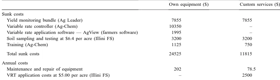
Table 1
Fixed costs of adopting SSCMa
Own equipment ($) Custom services ($) Sunk costs
Yield monitoring bundle (Ag Leader) 7855 7855
Variable rate controller (Ag-Chem) 10350 –
Variable rate application software — AgView (farmers software) 1995 – Soil sampling and testing at $6.4 per acre (Illini FS) 3200 3200
Training (Ag-Chem) 1125 750
Total sunk costs 24525 11815
Annual costs
Maintenance and repair of equipment 202 78.5
VRT application costs at $5.00 per acre (Illini FS) – 2500
aAll prices are in 1997 dollars. Sources: Illini FS Agricultural Cooperative, http://www.illinifs.com; Ag Leader, Ag Leader Technology,
http://www.agleader.com/; Farmer’s Software Association, http://www.farmsoft.com/; Ag-Chem, http://www.ag-chem.com/.
by the soil for the next crop.5 We assume no leaching or runoff of phosphorus and potassium as in Schnitkey et al. (1996). In the case of nitrogen we assume that 0.75 lbs of applied nitrogen are absorbed by a bushel of corn and that all excess nitrogen in the soil is po-tentially available for leaching (Barry et al., 1993).
We consider two approaches to adoption of SSCM, owner–purchase of all the necessary equipment or custom hiring of some services and purchase of the rest. The costs of both packages are shown in Table 1. All equipment prices are in 1997 dollars. Yield monitors and GPS units are typically purchased by farmers while custom services may be used for soil sampling, analyzing and mapping as well as vari-able rate fertilizer application. Under both approaches the cost of grid sampling at the 2.5 acre level is $6.4 per acre or $3200 for the 500 acres. We also assume that farmers purchase a yield monitoring bundle that includes a yield monitor with moisture sensors, a GPS receiver, field marker, mapping software, instal-lation and memory cards. This package is sold by Ag Leader for $7855. Farmers have the option of ei-ther purchasing the variable rate controller equipment themselves together with the application software for $12 345 or of hiring the services of a professional dealer for applying inputs at a varying rate in the field.
5This is a reasonable assumption since phosphorus and
potas-sium are not mobile nutrients in the soil. Unlike nitrogen they usually remain in the soil and contribute to environmental contam-ination only through soil erosion (Illinois Agronomy Handbook, 1998; Schnitkey et al., 1996).
The latter costs $5 per acre (Illini FS), i.e. $2500 for the 500 acres and is an annual cost. Finally, farmers adopting SSCM need to undergo training in the use of equipment. This is assumed to be a one-time sunk cost at the time of adoption. Annual costs of maintenance and repair are assumed to be 1% of the equipment cost.
Two alternative rates of discount are assumed, 5 and 10%, while the lifetime of the equipment is as-sumed to be 5 years. The total capital cost of the owner-purchased package is $24 525, while that of the custom-hired package for a 5-year period in present value terms (at a 5% discount rate) is $23 180. In an-nualized terms also, over a 5-year period with a 5% discount rate, the capital cost of the two packages is very similar — an owner-purchased package costs $5665 per annum, while a custom-hired package costs $5227 per annum. All equipment costs are assumed to decline in real terms by 5% per annum, while cost of custom hire services is assumed to decline by 3% per annum. Prices of nitrogen, phosphorus and potassium are assumed to be at their 1997 levels of $0.2 per lb, $0.24 per lb and $0.13 per lb, respectively.
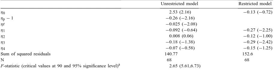
Table 2
Dickey–Fuller test for non-stationarity of the price process
Unrestricted model Restricted model
η0 2.53 (2.16) −0.13 (−0.72)
ηp−1 −0.26 (−2.16)
ηt −0.025 (−2.08)
η1 −0.092 (−0.64) −0.27 (−2.25)
η2 0.008 (0.06) −0.12 (−1.00)
η3 −0.18 (−1.38) −0.29 (−2.42)
η4 −0.07 (−0.58) −0.15 (−1.25)
Sum of squared residuals 140.77 152.6
N 68 68
F-statistic (critical values at 90 and 95% significance level)a 2.65 (5.61,6.73)
aCritical values for theτ-statistic at 90 and 95% significance levels are 2.4 and 2.8, respectively (Dickey and Fuller, 1981). Statistics
are in parenthesis.
process is non-stationary:
1Pt =η0+(ηp−1)Pt−1+ηtt+ I
X
i=1
ηi1Pt−i+εt
(14)
where1Pt =Pt−Pt−1and I is selected on the basis of the likelihood ratio test. A unit root test is conducted by comparing the sum of squared residuals from the unrestricted version in (14) and a restricted regression withηp−1 =0 andηt =0 using an F-test. The
re-sults of the F-test and aτ-test on the coefficientsηp−1 andηt are reported in Table 2. Both tests fail to reject
the null hypothesis of non-stationarity. We, therefore, assume that the output price process follows a geo-metric Brownian motion with an average growth rate αp and a standard deviation σp. Using data on real corn prices we estimateαp to be (−) 0.0146 andσp to be 0.223. Future prices are forecasted for a 25-year period using 1997 as the base year. These forecasted prices are used to forecast the discounted quasi-rent differential VT, if adoption were to be undertaken at
timeT =1, . . . ,25. A series of VT is estimated for
the 25 years under each of the alternative assumptions about the parameters of the soil fertility and soil qual-ity distributions. For each of these series we estimateα andσ to characterize the stochastic process followed by VT and determine the option value in (10).
4. Optimal timing of adoption
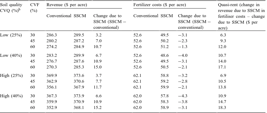
Table 3 shows the impact of alternative soil fertility and soil quality distributions on the per acre revenue,
fertilizer costs and quasi-rent differential with the two technologies, assuming a discount rate of 5%. The revenue and cost estimates presented in Table 3 are the discounted annual average for the first 5 years if adoption occurred atT =0. We find that adoption of SSCM leads to an increase in yields and therefore an increase in revenue for all soil fertility and quality dis-tributions considered here, although the extent of these gains varies with soil fertility and quality distributions. Revenue gains from adoption of SSCM increase as the average quality of the soil increases. These rev-enue gains also increase as the CV of the soil fertility and/or soil quality distribution increases.
Table 3
Average annual revenue gains and fertilizer costs with adoption of SSCMa
Soil quality CVQ (%)b
CVF (%)
Revenue ($ per acre) Fertilizer costs ($ per acre) Quasi-rent (change in revenue due to SSCM in fertiliser costs – change due to SSCM ($ per acre)
Conventional SSCM Change due to SSCM(SSCM−
conventional)
Conventional SSCM Change due to SSCM(SSCM−
conventional)
Low (25%) 30 286.3 289.5 3.2 52.6 49.5 −3.1 6.3
45 280.2 287.2 7.0 52.6 50.2 −2.3 9.3
60 274.2 284.9 10.7 52.6 51.2 −1.3 12.0
Low (40%) 30 283.2 289.9 6.7 52.6 48.6 −4.0 10.7
45 276.7 287.6 10.9 52.6 49.5 −3.1 14.0
60 270.3 285.3 15.0 52.6 50.5 −2.1 17.1
High (25%) 30 369.9 373.6 3.7 62.1 58.8 −3.2 6.9
45 362.9 370.6 7.7 62.1 59.2 −2.8 10.5
60 356.1 367.9 11.7 62.1 59.9 −2.1 13.8
High (40%) 30 367.3 373.9 6.6 62.0 57.8 −4.3 10.9
45 359.9 370.9 10.9 62.0 58.3 −3.8 14.7
60 352.9 368.1 15.2 62.0 58.9 −3.1 18.3
aSimulations done assuming a discount rate of 5%. Revenue and fertilizer costs are average of the discounted per acre values over the
5-year lifetime of equipment, if adoption were to occur atT =0.
bThe soil fertility level is represented by an average level of phosphorus of 30 lbs per acre and an average level of potassium of 200 lbs
per acre. Low soil quality indicates an average potential yield of 130 bushels per acre. High soil quality indicates an average potential yield of 165 bushels per acre. CVF refers to coefficient of variation of soil fertility distribution. CVQ refers to coefficient of variation of soil quality distribution.
to improved soil quality diminishes as soil quality rises. Hence, the increase in input applications on the increased proportion of high soil quality plots is less than the reduction in input applications on the in-creased proportion of low quality plots and therefore total variable costs decrease with adoption.
Although input-cost savings from adoption decrease as the variability of the soil fertility and soil quality distributions increase, these costs are more than offset by the corresponding gain in revenue. The quasi-rent differential due to adoption (as in (6)) increases as the average level of soil quality increases and as the variability in soil fertility and/or soil quality increases. The discounted average annual per acre quasi-rent dif-ferential varies between $6.3 per acre on low quality relatively uniform soil to $18.3 per acre on the high quality soils with high variability in soil conditions.
With the same fixed costs for all soil conditions, investment in SSCM is more likely to be profitable on farms with high soil quality and high variability in soil fertility and quality. Hence, as shown in Table 4, adoption is not profitable according to the NPV rule on soil distributions with low average soil quality and relatively uniform soil conditions. On soil
distribu-tions that have higher quality levels and high CV, the NPV rule recommends immediate investment. Since the annualized costs of the custom hire package are very close to those of the owner-purchased package, the NPV rule does not indicate a difference in the adoption decision between the two packages in most cases.
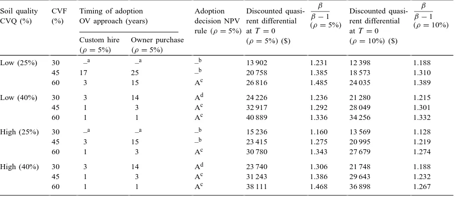
disin-Table 4
Optimal adoption decision under alternative soil fertility and soil quality distributions Soil quality
CVQ (%)
CVF (%)
Timing of adoption OV approach (years)
Adoption decision NPV rule(ρ=5%)
Discounted quasi-rent diffequasi-rential atT =0
(ρ=5%)($)
β β−1
(ρ=5%)
Discounted quasi-rent diffequasi-rential atT =0
(ρ=10%)($)
β β−1
(ρ=10%)
Custom hire
(ρ=5%)
Owner purchase
(ρ=5%)
Low (25%) 30 –a –a –b 13 902 1.231 12 398 1.188
45 17 25 –b 20 758 1.385 18 573 1.310
60 3 15 Ac 26 816 1.485 24 035 1.389
Low (40%) 30 3 14 Ad 24 226 1.236 21 280 1.215
45 1 3 Ac 32 917 1.292 28 049 1.301
60 1 1 Ac 40 889 1.336 34 256 1.332
High (25%) 30 –a –a –b 15 236 1.160 13 569 1.128
45 3 15 –b 23 415 1.275 20 995 1.219
60 1 3 Ac 30 780 1.343 27 679 1.274
High (40%) 30 3 14 Ad 23 740 1.306 21 748 1.188
45 1 3 Ac 31 243 1.386 29 643 1.232
60 1 1 Ac 38 111 1.468 36 898 1.267
aAdoption is not profitable in the next 25 years.
bAdoption is not profitable att=0 according to the NPV rule. cAdoption att=0 is profitable according to the NPV rule.
dAdoption of custom hire services is profitable but not owner purchase of SSCM equipment.
CVF refers to coefficient of variation of soil fertility distribution. CVQ refers to coefficient of variation of soil quality distribution.
centives for investment due to price uncertainty and irreversibility.
As the average level of soil quality decreases and CV of soil quality and soil fertility levels decrease, the OV approach recommends that it is optimal to wait rather than invest immediately as suggested by the NPV rule, particularly in owner purchase of equipment. The optimal delay in adoption ranges from 3 to 25 years. Although the discounted expected quasi-rent differential with the adoption of the cus-tom hire-packaged and the owner-purchased package is the same, the threshold value V˜T at which
im-mediate adoption is optimal is much higher for the owner-purchased package because the sunk capital costs (KT) are larger. Hence, the optimal timing for
adoption through owner purchase is considerably later than through custom hire. Both the NPV rule and the OV approach indicate that adoption is not profitable in the next 25 years on soil distributions with CV of soil fertility of 30% and CV of soil quality of 25%.
In some cases, the OV approach recommends de-layed adoption while the NPV rule does not indicate that adoption would be profitable. This is the case on low quality soils and 25% CV in soil quality with
medium variability in soil fertility(CV=45%). Here adoption at t = 0 is not profitable according to the NPV rule but the OV approach suggests that it can be profitable to adopt SSCM with custom hiring after 17 years on high quality soil and after 25 years on low quality soil. This is because the OV approach incor-porates the decline in fixed costs, the variability in VT
over time and the flexibility in the timing of adoption. An increase in the discount rate to 10% reduces (β/(β−1))marginally as shown in the last column in Table 4. This would tend to hasten adoption of SSCM. However, it also lowers the discounted value of the quasi-rent differential marginally (Column 8 of Table 4). Hence the discount rate has little impact on the adoption decision under the NPV or the OV approach.
5. Implications of SSCM for pollution control
Table 5
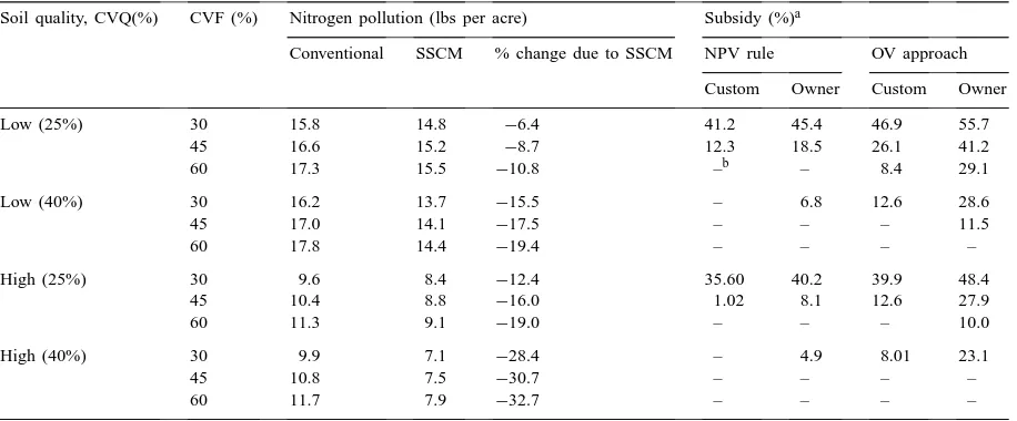
Nitrogen pollution reduction and cost-share subsidy requirements
Soil quality, CVQ(%) CVF (%) Nitrogen pollution (lbs per acre) Subsidy (%)a
Conventional SSCM % change due to SSCM NPV rule OV approach Custom Owner Custom Owner
Low (25%) 30 15.8 14.8 −6.4 41.2 45.4 46.9 55.7
45 16.6 15.2 −8.7 12.3 18.5 26.1 41.2
60 17.3 15.5 −10.8 –b – 8.4 29.1
Low (40%) 30 16.2 13.7 −15.5 – 6.8 12.6 28.6
45 17.0 14.1 −17.5 – – – 11.5
60 17.8 14.4 −19.4 – – – –
High (25%) 30 9.6 8.4 −12.4 35.60 40.2 39.9 48.4
45 10.4 8.8 −16.0 1.02 8.1 12.6 27.9
60 11.3 9.1 −19.0 – – – 10.0
High (40%) 30 9.9 7.1 −28.4 – 4.9 8.01 23.1
45 10.8 7.5 −30.7 – – – –
60 11.7 7.9 −32.7 – – – –
aPercentage of the total fixed costs (reported in Table 1) for owner purchase and custom hire for 5 years. bNo subsidy is required.
levels under both conventional technology and SSCM are higher on soil distributions characterized by low average soil quality. As the variability in soil fertility increases, input applications increase for reasons ex-plained above. This results in increased nitrogen pol-lution under both technologies. However, the increase is lower under SSCM as compared to conventional production practices. Hence the reduction in pollution levels is much higher on soil distributions with more variable soil fertility. Adoption of SSCM also leads to larger levels of pollution reduction on soil quality distributions with greater variability. An increase in average soil quality raises input uptake more than input application rates and therefore reduces nitrogen pollution with either technology. The reduction in nitrogen pollution with adoption on distributions with high average soil quality ranges from 12.4 to 32.7%, while on distributions with low average soil quality it ranges from 6.4 to 19.4%.
The analysis above shows that the reduction in nitro-gen pollution is largest on soil distributions with high average quality and medium to high variability in soil conditions (Table 5). These are also the soil distribu-tions on which immediate adoption could occur even under the option value approach as shown in Table 4. Hence, on these soil conditions, there is a possibility of realizing a complementarity in the dual goals of
of the sunk costs of adoption. This difference is much greater under the OV approach that accounts for the greater irreversibility of the owner-purchased package relative to the custom-hired one. Table 5 shows that required subsidy rates on owner purchase could be as high as 56%, while those on custom hiring are only 45%. Hence, to achieve the same level of pollution reduction it would be more cost-effective to subsidize adoption of SSCM through custom hire rather than owner purchase.
6. Conclusions
This paper applies an option-pricing model to ana-lyze the impact of uncertainty about output prices and expectations of declining fixed costs on the optimal timing of investment in SSCM and the variability in this impact across heterogeneous soil conditions. It also undertakes an ex-ante assessment of the impli-cations of a value of waiting to invest in SSCM for the design of a cost-share subsidy policy that seeks to reduce pollution by accelerating adoption. The paper thereby provides a rationale for the currently observed low rates of adoption of SSCM and why farmers prefer to wait before adopting. Numerical simulations show that the NPV rule predicts that immediate adoption is profitable under most of the soil conditions simulated here (except where soil quality levels are very low and their distribution is relatively uniform). How-ever, recognition of the option value of investment indicates that it is preferable to delay investment in SSCM for at least 3 years unless average soil quality levels are high and soil conditions are very variable. Delays in adoption are likely to be longer on fields with lower average soil quality and relatively uniform conditions.
The reduction in pollution is relatively large on soil quality distributions characterized by high levels and high variability in soil fertility and quality. These are also the soil distributions on which immediate adoption is profitable even under the OV approach and without any cost-share subsidy. On other soil dis-tributions, the cost-share subsidy rates required to in-duce immediate adoption under the OV approach are larger than would have been required under the NPV rule. The paper also shows that the cost-share sub-sidy required to induce adoption of the custom-hired
package is substantially lower than that required for inducing owner purchase, particularly under the OV approach. It would, therefore, be more cost-effective to achieve a given level of pollution reduction by sub-sidizing custom hire rather than owner purchase of equipment.
Acknowledgements
This research has been funded by the Illinois Council for Food and Agricultural Research.
References
Babcock, B.A., Pautsch, G.R., 1998. Moving from uniform to variable fertilizer rates on Iowa corn: effects on rates and returns. J. Agric. Resourc. Econ. 23 (2), 385–400.
Barry, D.A.J., Goorahoo, D., Goss, M.J., 1993. Estimation of nitrate concentration in groundwater using a whole farm nitrogen budget. J. Environ. Qual. 22, 767–775.
Caswell, M.F., Zilberman, D., Casterline, G., 1993. The diffusion of resource-quality-augmenting technologies: output supply and input demand effects. Nat. Resourc. Model. 7 (4), 305–329. Chin, K.C., 1997. Soil sampling for nitrate in late spring.
Unpublished Ph.D. Dissertation. Department of Agronomy, Iowa State University, Ames, IA.
Committee on Long Range Soil and Water Conservation, 1993. Soil and Water Quality: An Agenda for Agriculture. National Academy Press, Washington, DC.
Daberkow, S.G., McBride, W.D., 1998. Adoption of precision agriculture technologies by US corn producers. J. Agribusiness 16 (2), 151–168.
Dai, Q., Fletcher, J.J., Lee, J.G., 1993. Incorporating stochastic variables in crop response models: implications for fertilization decisions. Am. J. Agric. Econ. 75, 377–386.
Dickey, D.A., Fuller, W.A., 1981. Likelihood ratio statistics for autoregressive time series with a unit root. Econometrica 49 (4), 1057–1072.
Dixit, A.K., Pindyck, R.S., 1994. Investment Under Uncertainty. Princeton University Press, Princeton, NJ.
Frank, M.D., Beattie, B.R., Embleton, M.E., 1990. A comparison of alternative crop response models. Am. J. Agric. Econ. 72 (3), 597–603.
Illinois Agronomy Handbook, 1998. Cooperative Extension Service. Department of Crop Sciences, University of Illinois at Urbana-Champaign.
Khanna, M., Epouhe, O.F., Hornbaker, R., 1999. Site-specific crop management: adoption patterns and trends. Rev. Agric. Econ. 21 (2), 455–472.
Olson, K.R., Lang, J.M., 1994. Productivity of Newly Established Illinois Soils, 1978–1994. Supplement to Soil Productivity in Illinois. Department of Agronomy, University of Illinois at Urbana-Champaign, IL.
Purvis, A., Boggess, W.G., Moss, C.B., Holt, J., 1995. Technology adoption decisions under irreversibility and uncertainty: an ex-ante approach. Am. J. Agric. Econ. 77, 541–551. Ray, D.E., Richardson, J.W., De La Torre Ugarte, D.G.,
Tiller, K.H., 1998. Estimating price variability in agriculture: implications for decision makers. J. Agric. Appl. Econ. 30 (1), 21–33.
Schnitkey, G.D., Hopkins, J.W., Tweeten, L.G., 1996. An economic evaluation of precision fertilizer applications on corn–soybean fields. In: Robert, P.C., Rust, R.H., Larson, W.E. (Eds.), Proceedings of the Third National Conference on Precision Agriculture, June 23–26, 1996. American Society of Agronomy. Swinton, S.M., Lowenberg-DeBoer, J., 1998. Evaluating the profitability of site-specific farming. J. Prod. Agric. 11 (4), 439–446.
Thrikawala, S., Weersink, A., Kachnoski, G., Fox, G., 1999. Economic feasibility of variable rate technology for nitrogen on corn. Am. J. Agric. Econ. 81 (4), 914–927.
USDA, 1965–1998. Agricultural Statistics. National Agricultural Statistics Service. Government Printing Office, Washington, DC (Annual Issues, 1965–98). http://www.usda.gov/nass/pubs/ histdata.htm.
USDA, 1999. In: Harwood, J. (202-694-5310), Heifner, R., Coble, K., Perry, J., Somwaru, A. (Eds.), Managing Risk in Farming: Concepts, Research, and Analysis. Agricultural Economic Report 774. Market and Trade Economics Division, Economic Research Service, US Department of Agriculture. Watkins, K.B., Lu, Y., Huang, W., 1998. Economic and
environ-mental feasibility of variable rate nitrogen fertilizer application with carryover effects. J. Agric. Resourc. Econ. 23 (2), 401– 426.