SPEEDING UP COARSE POINT CLOUD REGISTRATION BY
THRESHOLD-INDEPENDENT BAYSAC MATCH SELECTION
Z. Kang a*, R. Lindenbergh b, S. Pu c a
Department of Remote Sensing and Geo-Information Engineering, School of Land Science and Technology, China University of Geosciences, 29 Xueyuan Road, Haidian District, Beijing 100083, China - [email protected]
b
Chair Optical and Laser Remote Sensing, Dept. Geosciences and Remote Sensing, Fact. Civil Engineering and Geosciences, Delft University of Technology, Stevinweg 1, 2628 CN, Delft, The Netherlands - [email protected]
c
Beijing Tovos Technology Co., Ltd, Unit 1602, TOP Building Tower B, Haidian Dajie No.3, Haidian District. Beijing, China Commission V, WG V/3
KEY WORDS: BaySAC, Convergence evaluation, Hypothesis set, Inlier probability, Point cloud registration, RANSAC
ABSTRACT:
This paper presents an algorithm for the automatic registration of terrestrial point clouds by match selection using an efficiently conditional sampling method -- threshold-independent BaySAC (BAYes SAmpling Consensus) and employs the error metric of average point-to-surface residual to reduce the random measurement error and then approach the real registration error. BaySAC and other basic sampling algorithms usually need to artificially determine a threshold by which inlier points are identified, which leads to a threshold-dependent verification process. Therefore, we applied the LMedS method to construct the cost function that is used to determine the optimum model to reduce the influence of human factors and improve the robustness of the model estimate. Point-to-point and Point-to-point-to-surface error metrics are most commonly used. However, Point-to-point-to-Point-to-point error in general consists of at least two components, random measurement error and systematic error as a result of a remaining error in the found rigid body transformation. Thus we employ the measure of the average point-to-surface residual to evaluate the registration accuracy. The proposed approaches, together with a traditional RANSAC approach, are tested on four data sets acquired by three different scanners in terms of their computational efficiency and quality of the final registration. The registration results show the st.dev of the average point-to-surface residuals is reduced from 1.4 cm (plain RANSAC) to 0.5 cm (threshold-independent BaySAC). The results also show that, compared to the performance of RANSAC, our BaySAC strategies lead to less iterations and cheaper computational cost when the hypothesis set is contaminated with more outliers.
* Corresponding author
1. INTRODUCTION
Terrestrial laser scanning (TLS) is effectively used in urban mapping for applications like as-built documentation, change detection, 3D reconstruction of architectural details and building facades. However, one of the biggest problems encountered while processing the scans is the so-called registration step in which rigid transformation parameters (RTPs) are determined in order to align scans obtained from different scan positions into one common coordinate system. RTPs are computed from minimizing distances between common points, obtained by correspondence tracking, in scenes sampled from different viewpoints. In general two registration goals are distinguished, coarse and fine registration. A coarse registration of sufficient quality is typically needed as input for a successful fine registration (Vosselman & Maas, 2010). This paper is focused on coarse registration.
Coarse registration should be able to compute an initial estimate of the transformation between two point clouds that are quite far apart. A well-known approach is to compute motion invariant features (or descriptors) for both sets and consecutively match these features. The feature extraction and matching step is generally approached in three different ways: Manual point-based matching, target-point-based matching and feature-point-based
matching. However, existing fully automated approaches may only work in certain contexts.
Besides differing on the type of descriptors used, coarse registration algorithms also differ on the matching methods used to establish correspondences between scans (e.g. ordinary Least Squares adjustment, Genetic Algorithms (Brunnström & Stoddart, 1996), Principal Component Analysis ‘‘PCA’’ (Chung & Lee, 1998) or RANdom Sample And Consensus ‘‘RANSAC’’ (Fischler & Bolles, 1981)). Kang et al. (2009) proposed an iterative algorithm, using Lease Squares adjustment, for optimal transformation parameters estimation. Akca (2010) achieved the parameter estimation using a Generalized Gauss-Markov model. Grant et al. (2012) proposed a point-to-plane fine registration approach that also uses a General Least Squares adjustment model.
In many cases RANSAC is used to automatically remove false matches. However, the original RANSAC algorithm assumes constant prior probabilities for all data points and chooses hypothesis sets at random, which leads to many iterations and high computational costs as many hypothesis sets will be contaminated with outliers.
Therefore, the scope of this paper is focused on improving the efficiency of coarse matching by improving on the RANSAC The International Archives of the Photogrammetry, Remote Sensing and Spatial Information Sciences, Volume XLI-B5, 2016
paradigm, The SIFT-based reflectance image matching method (Kang et al., 2009) is employed to determine initial 3D correspondences. For robust estimation of transformation parameters from 3D correspondences contaminated by outliers, we implement a conditional sampling method – optimized BaySAC (Kang et al., 2014) to always select the minimum number of data required with the highest inlier probabilities as hypothesis set. Moreover, LMedS method is used to construct the cost function that is used to determine the optimum model. We evaluate the results of the optimized BaySAC strategy compared to a traditional RANSAC approach both by considering the required computational efforts and by comparing the quality of the resulting registration. For the latter, we compare the RMSEs of the distances between matching points in the final inlier set and, in addition, evaluate the Euclidean distances between the transformed points in the analyzed scan to the surface fitted to the fixed scan.
2. DETERMINATION OF THE PRIOR INLIER PROBABILITIES OF DATA POINTS
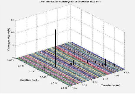
Determining the proper prior inlier probability is important for the BaySAC algorithm. We implemented the statistical testing process proposed in (Kang et al., 2014), which is generic and can be applied to any BaySAC problem. The process is implemented using a histogram that illustrates the distribution of the discrete hypothesis model parameter sets that are computed during the different iterations and the degree of convergence of each candidate parameter set that describes how the other sets converge to it. The degree of convergence of a bin in the histogram is calculated as the number of parameter sets in that bin divided by the total number of parameter sets.
Our presented strategy is based on a histogram to dynamically evaluate the convergence of the hypothesis parameters sets during the hypothesis testing process (Fig.1 shows a histogram to evaluate the convergence of the rigid transformation parameters. Different convergent cluster of the hypothesis sets will be presented in the histogram. We select the oldest parameter set as the reference point for each convergent cluster of parameter sets. The more the hypothesis sets converge to a cluster, the more possible is it that the reference parameters set of the cluster is correct. Therefore, we present the convergence degree of a cluster to evaluate the correct possibility. The convergence degree is a percentage which describes the number
of sets converge to a parameters sets cluster. It is calculated by dividing the number of the hypothesis sets in the cluster by the total number of hypothesis sets.
In this paper, the rigid transformation model in point cloud registrationis used as the hypothesis models.
The hypothesis testing process starts with a RANSAC strategy which chooses initial data sets at random. After that, during each iteration, the distribution of the hypothesis parameters sets is updated by adding the parameters set corresponding to the newly evaluated hypothesis sets. If a newly added set doesn’t converge to any existing cluster, it will be regarded as a new cluster in the distribution. Else, the number of solutions in an existing cluster is increase by one and the convergence degree of the different clusters is updated accordingly.
When the degree of convergence of a cluster in the distribution of parameter solutions reaches a predefined threshold, the first hypothesis set in that cluster is used to determine the prior inlier probabilities of the data points according Eq. (1):
represents the predefined threshold for outlier identification, which is set as five times the point precision.3. PROBABILITY UPDATING
After determining the prior inlier probabilities of each corresponding pair, Eq. (2) (Kang et al., 2014) is employed to update the inlier probabilities during consecutive iterations:
data points used in iteration t of the hypothesis testing process,
Pt-1(i
I) and Pt(i
I) denote the inlier probabilities for datapoint i during iterations t-1 and t, respectively, k is the number of points consistent with the model during a test, and D is the total number of data points.
4. CONSTRUCTION OF THE COST FUNCTION USING LMEDS
We applied the LMedS method (Rousseeuw & Leroy, 1987) to construct the cost function that is used for determining the optimum model to reduce the influence of human factors and improve the robustness of the model estimate.
We first randomly select a subset of corresponding points from the samples to calculate the model parameters and then calculate the deviation (i.e., distances between corresponding points) of all the other sample points with respect to the model. We use the equation as follows to calculate the deviation in the Figure 1 2D histogram of parameter sets corresponding to
different hypothesis sets
middle of all the model deviations, which is called the Med number of data points used to test the model parameter. We used Med deviation to replace the number of inlier points complying with the hypothesis model as the criteria to determine the optimum model. After the iterative process of the hypothesis test is finished, we select the model with the smallest Med deviation as the optimum model.
5. RESULT EVALUATION
Accuracy is of great importance for point cloud registration. Therefore, various error metrics have been defined to measure the registration accuracy of point clouds (Simon, 1996; Maas, 2000; Rusinkiewicz & Levoy, 2001). These include the change in rotation angle and/or translation vector, the distances between corresponding points and the distances between points and their corresponding surfaces. Among them, point-to-point and point-to-surface error metrics are most commonly used, both of which are utilized in this paper. As the registration process is implemented using 3D corresponding points, we naturally use the st.dev of the distances between corresponding points in the first scan and their transformed matches from the second scan, to evaluate the quality of the registration results. However, the error evaluated as a point to point difference between two scans after registration in general consists of at least two components, a random measurement error component and a systematic error component as a result of a remaining error in the found rigid body transformation. Still, in most publications the quality of a registration is expressed in terms of standard deviations, which assumes an underlying normal distribution. Thus we employ the measure of the average point-to-surface residual, introduced by (Lindenbergh & Pfeifer, 2005) to evaluate the registration accuracy.
5.1 Distances between corresponding points
The first method to evaluate the quality of the resulting registration is by considering the distances at corresponding points as follows. Applying the methods on the initial set of corresponding pairs results in general different sets of correct correspondences. As indicated before, the correct correspondences are used to estimate a final rigid body transformation TR using least squares. The resulting transformation TR is applied to each inlying corresponding point in the second scan. Finally the st.dev of the distances between corresponding points in the first scan and their transformed matches from the second scan is determined. Advantage of this approach is that it is expected that matches are found throughout the overlap between the two scans. 5.2. Average point-to-surface residual
The error evaluated as a point to point difference between two scans after registration normally comprises at least two components, i.e. random measurement error and registration error. As errors in the computed transformation parameters lead
to non-random differences between the fixed and transformed scans, we consider the registration error as systematic.
Random errors are also known as compensating errors, since they tend to partially cancel themselves in a series of measurements. In this paper, we implement the U test (Lehman & Romano, 2005) to estimate the normality of the distribution of the residuals. The formula to compute U value in terms of the skewness or kurtosis of the distribution is as follow.
represent kurtosis and its st.dev.
If U1 and U2 both satisfy the following condition, the distribution is regarded as normal.
96 difference is expected to approach the real registration error. First, the surface representations, e.g. plane and curve, are obtained from the first scan using the RANSAC algorithm. We then compute the distances between the transformed points (from the second scan) to the surface of the fixed reference, the first scan. For the purpose of reducing the effect of random measurement noise, the point-to-surface residuals are averaged to a regular grid spanned over the considered surface segment. The average point-to-surface residual per cell is expected to reduce the random error so that this residual approaches the real registration error.
6. EXPERIMENT AND ANALYSIS
The performances of the threshold-independent BaySAC algorithm was evaluated on real datasets in terms of both registration accuracy and computational efficiency.
6.1. Description of the test data
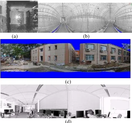
Four datasets are considered, acquired respectively by the 3D SwissRanger camera, by the LMS-Z620 and VZ-400 laser scanners from RIEGL, as well as by the FARO LS 880 laser scanner (Fig.2). The SwissRanger dataset consists of two point clouds sampling the indoor environment of a building of the Aerospace Engineering Faculty of Delft University of Technology, The Netherlands. The RIEGL LMS VZ-400 dataset comprises six point clouds acquired in a subway tunnel in Shanghai, China. The FARO dataset consists of two point clouds of an office environment, while the RIEGL LMS-Z620 dataset consists of two point clouds, capturing a simple building in construction on the campus of Capital Normal University in Beijing, China. Tab. 1 describes the test point clouds. Note that both the angular resolution and the range accuracy of the SwissRanger data are much lower than those of normal laser scanners.
Two robust strategies, i.e. RANSAC, BaySAC-LMedS, were respectively utilized to prune false correspondences.
6.2. Registration accuracy
As presented in Section 5, the registration accuracies of RANSAC and BaySAC-LMedS on four datasets were evaluated using two measures, the average distance between inlier correspondences after registration and the average point-to-surface residual.
6.2.1. Average point-to-point distance
Fig.3 shows that a certain number of correspondences (e.g. 5 of Dataset 1) were identified for each dataset as check points. Tab.2 lists the evaluation of registration accuracies in terms of the average distance between the selected correspondences after registration. BaySAC-LMedS achieved overall higher accuracy (the average RMSs 8.1 mm) compared with the performance of the plain RANSAC (the average RMSs 22.9 mm).
6.2.2. Average transformed-point-to-analyzed-surface residual per cell
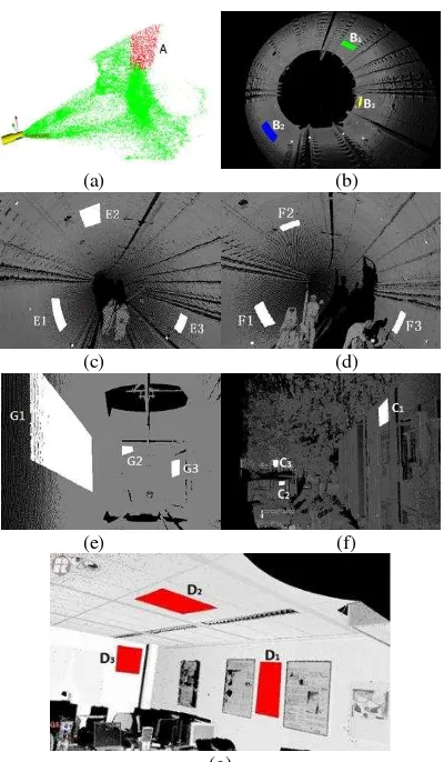
For the purpose of registration quality evaluation we selected ten planar segments from Datasets 1, 2, 3 and 4 and nine curved-surface segments from Dataset 2. These segments are visualized in Fig.5 To evaluate the registration error, we computed the Euclidean distances between the transformed points in the analyzed scan and the surface fitted to the fixed
scan. Non-zero distances are mainly caused by three factors: measurement errors, surface fitting errors and registration errosr. The first factor is believed to be random, therefore the influence of the two other factors are analyzed in the following sections. 1) Average point-to-fitted-surface residuals after surface fitting
(a) (b)
(c)
(d)
Figure 2. Experimental datasets visualized as panoramic 2D images. The grey values indicate intensity. (a) Dataset 1; (b) Dataset 2; (c) Dataset 3; (d) Dataset 4.
Point Cloud Scan Angular
Resolution Range Accuracy
Dataset 1 0.24 ±10 mm
Dataset 2 0.046 ±2 mm
Dataset 3 0.0469 ±10 mm
Dataset 4 0.036 ±3 mm
Table 1. Description of the test point clouds.
(a) (b)
(c) (d)
(e) (f)
(g)
Figure 3. Check points. (a) Dataset 1; (b) Dataset 2(Point cloud I~II); (c) Dataset 2 (Point cloud II-III); (d) Dataset 2 (Point cloud III-IV); (e) Dataset 2 (Point cloud pair V-VI);
(f) Dataset 3; (g) Dataset 4.
(a) (b)
(c) (d)
Figure 4. The histograms of point-to-surface residuals of the fitted surfaces. (a) Dataset A; (b) Dataset B1; (c) Dataset C1; (d) Dataset 2 D1.
As proposed in Section 5, RANSAC was implemented to fit points from selected segments from the first scan to surface representations. To evaluate the fitting error, we computed the point-to-surface residuals per segment.
Fig.4 shows the histograms and spatial distributions of the point-to-surface residuals for the fitted surfaces (e.g. A, B1, C1 and D1) of the four datasets.
As proposed in Section 5.2, we implemented the U test to estimate the normality of the distribution of the residuals. Tab. 4 lists the U values computed in terms of skewness and kurtosis of the residual distributions of nineteen fitted surfaces.
From Tab. 3 we can know that all U1 and U2 values are less than the threshold value 1.96 of U0.05, which strongly indicates that the distribution of point-to-surface residuals of the fitted surface is normal.
The average point-to-surface residuals are given in Tab 4. All signed average point-to-surface residuals are below 1 mm, which proves that the signed point-to-surface residuals can partially cancel themselves after averaging, compared with the RMS of the point-to-surface residuals.
2) Points to surface registration residuals
To evaluate the registration error, we computed the Euclidean distances between the transformed points in the analyzed scan to the surface fitted to the fixed scan. Fig.6 shows the histograms of these distances. Compared to Fig. 4, in Fig. 6 obvious shifts from the origin are visible, which we interpret as being caused by registration errors because the surface fitting error is proven to be random.
Afterwards, we superimposed a regular grid with an edge length of 10cm on the selected surface segment and calculated the average point-to-surface difference for each cell. Fig.7 ( Segment D1) shows that both of the magnitudes and signs of the average point-to-surface differences per cell are non-random and are expected to approach the real registration error. The spatial distribution of the residuals also appears systematic (Fig.7), for instance most larger differences occur in the bottom left part of Fig.7(a). Fig.7(b) shows a distribution of differences with smaller absolute values, compared to the distributions shown in Fig.7(a).
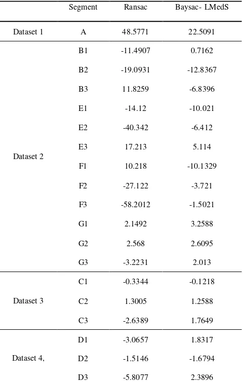
The average differences between the transformed points from the registered scan and the reference surface are shown in Tab.5. From The two different strategies BaySAC-LMedS, on the whole, achieved registrations with the smaller residuals (average
Figure 5. Selected surface segments for registration quality evaluation. (a) Dataset 1; (b) Dataset 2 (Point cloud pair I-II); (c) Dataset 2 (Point cloud pair II-II-II); (d) Dataset 2
Table 2. The evaluation of registration accuracy in terms of the average point-to-point distance
residual 4.8mm), while the average residual of RANSAC is 14.2 mm.
6.3. Computational efficiency
Hypothesis set evaluation is an iterative process, so the calculational efficiency of the proposed strategies was evaluated in terms of the number of iterations and computation time. As described in Section 2, the BaySAC- LMedS strategy consists
of two parts, i.e. the random part (BaySAC- LMedS -Random) and the BaySAC part. The random part consists of the iterations implemented with a RANSAC strategy, during which the inlier probabilities of the different correspondences are determined as well.
As shown in Tab.6, the ratio between the number of inliers and the number of possible correspondences in Dataset 1 reaches 81%. The number of iterations for RANSAC varies from 6 to
(a)
(b)
Figure 7. The statistical histograms and spatial distributions of average point-to-surface residuals per cell (Segment D1). (a) BaySAC- LMedS; (b) RANSAC.
Table 5. Average point to surface residuals (non-random)
Segment Ransac Baysac-LMedS
Dataset 1 A 48.5771 22.5091
Dataset 2
B1 -11.4907 0.7162
B2 -19.0931 -12.8367
B3 11.8259 -6.8396
E1 -14.12 -10.021
E2 -40.342 -6.412
E3 17.213 5.114
F1 10.218 -10.1329
F2 -27.122 -3.721
F3 -58.2012 -1.5021
G1 2.1492 3.2588
G2 2.568 2.6095
G3 -3.2231 2.013
Dataset 3
C1 -0.3344 -0.1218
C2 1.3005 1.2588
C3 -2.6389 1.7649
Dataset 4,
D1 -3.0657 1.8317
D2 -1.5146 -1.6794
D3 -5.8077 2.3896
Segment
Point-to-surface residual Mean Value Standard deviation
Dataset 1 A 0.4531 0.2872
Dataset 2
B1 -0.054 0.11
B2 0.011 0.1
B3 0.0412 0.073
E1 0.0121 1.2014
E2 0.0945 0.7413
E3 0.0114 1.4575
F1 0.0079 0.0016
F2 0.2605 1.5711
F3 -0.0352 0.6751
G1 -0.2202 0.0388
G2 0.0103 0.0055
G3 -0.009 0.0038
Dataset 3
C1 -0.054 0.06
C2 0.0125 0.06
C3 -0.0072 0.0042
Dataset 4,
D1 -0.023 0.045
D2 0.0261 0.063
D3 0.0087 0.031
Table 4. The average point to surface residuals
(a) (b)
(c) (d)
Figure 6. The histograms and spatial distributions of the distance between the transformed points and the surface fitted to the points in the fixed scan. (a) Segment A; (b) Segment B1; (c) Segment C1; (d) Segment D1.
18. In attempts No. 1, 2, 7, 8, as presented in Section 2, the number of iterations for RANSAC is so small that the BaySAC-LMedS process failed in the determination of initial inlier probabilities of data points before the RANSAC process ended, therefore the BaySAC-LMedS degraded to a RANSAC process. The total number of iterations for BaySAC-LMedS varies from 2 to 11. The results show that, although the numbers of consumed iterations of BaySAC-LMedS is smaller than those of RANSAC as a whole, the differences are not so obvious due to the high percentage of inliers.
The percentage of inliers in Dataset 2 (e.g. point cloud pair I-II) reduces to 38% (Tab.6). The number of iterations for RANSAC varies between 283 and 437. The random part of BaySAC-LMedS takes between 4 and 26 iterations. As presented in Section 2, after the determination of the initial inlier probability
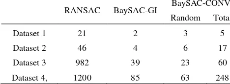
for each correspondence, the strategy of hypothesis set evaluation changes from RANSAC to BaySAC. Therefore, the total number of iterations, compared to those for a plain RANSAC strategy, sharply reduces to the range from 14 to 76. The results show that, although the number of possible correspondences is only 61 (Tab.6), the decrease of percentage of inliers leads to large differences between the performance of RANSAC and BaySAC-LMedS. When the percentage of inliers for Dataset 3 and 4 reduces further to 23% and 25%, the computational efficiency of RANSAC becomes much lower compared to BaySAC-LMedS. Tab. 6 compares the different statistics for the evaluated strategies. The average consumed time of the three strategies is listed in Tab. 7. As shown in Tab. 7, the random parts of the time consumed by BaySAC-LMedS was to determine the prior inlier probabilities of data points, which are the core of BaySAC-CONV.
After the determination of the prior inlier probabilities, the use of BaySAC remarkably reduced the computational time needed to find a good model compared with the time consumed by
In this paper, we have proposed conditional sampling algorithm for point cloud registration using the threshold-independent BaySAC framework. The measure of the average point-to-surface residual was employed to evaluate the registration accuracy for the purpose of reducing the random measurement error and thus approaching the real registration error.
The proposed algorithms were implemented and evaluated on four TLS data sets in terms of their computational efficiency and the quality of the registration results. The results show that, compared to the performance of the original RANSAC framework, the computational efficiency of BaySAC-LMedS scales with the percentage of inliers. The smaller this percentage, the higher the computation efficiency gain of BaySAC-LMedS on RANSAC. When the percentage of inliers becomes very large (e.g. 81%), the BaySAC-LMedS strategy may fail and thus degrades to a RANSAC process. The registration results also
indicate that, among the two different considered strategies, BaySAC-LMedS achieves the highest registration quality on all experimental datasets.
The proposed algorithm aims at robustly estimating a single transformation between two scans. Future work will consider how BaySAC-LMedS can be applied for the co-registration of multiple point clouds in the simultaneous estimation of multiple transformations.
REFERENCES
Akca, D., 2010. Co-registration of Surfaces by 3D Least Squares Matching. Photogrammetric Engineering and Remote Sensing, 76(3), pp.307-318.
Brunnström, K., Stoddart, A., 1996. Genetic algorithms for free-form surface matching. In: Proc. International Conference of Pattern Recognition, Vienna, pp.689-693.
Chung, D., Lee, Y.D.S., 1998. Registration of multiple-range views using the reverse calibration technique. Pattern Recognition,31 (4), pp.457–464.
Fischler, M.A. and Bolles, R.C, 1981. Random Sample Consensus: A Paradigm for Model Fitting with Applications to Image Analysis and Automated Cartography, Communications of the ACM, 24,pp.381–395. doi:10.1145/358669.358692. Grant, D., Bethel, J., Crawford, M., 2012. Point-to-plane registration of terrestrial laser scans. ISPRS Journal of Photogrammetry and Remote Sensing,72, pp. 16–26.
Kang, Z., Li, J., Zhang, L., Zhao, Q., Zlatanova, S., 2009. Automatic Registration of Terrestrial Point Clouds using Reflectance Panoramic Images, Sensors, 9, doi: 10.3390/sensors. Kang, Z., Zhang, L., Wang, B., Li, Z. and Jia, F., 2014. An optimized BaySAC algorithm for efficient fitting of primitives Possible Correspondences I/C ratio Iterations
(RANSAC)
Table 6. Computational efficiencies of the proposed strategies.
Average consumed time (millisecond)
RANSAC BaySAC-GI BaySAC-CONV
Random Total
Dataset 1 21 2 3 5
Dataset 2 46 4 6 17
Dataset 3 982 39 23 60
Dataset 4, 1200 85 63 248
Table 7. Computational efficiency comparison (iterations)
in point clouds, IEEE Geoscience and Remote Sensing Letters, 11(6), pp.1096–1100.
Lehman, E. L., and J. P. Romano, 2005. Testing Statistical Hypotheses. New York: Springer,,pp. 786.
Lindenbergh, R., Pfeifer, N., 2005. A statistical deformation analysis of two epochs of terrestrial laser data of a Lock, Proceedings of the 7th Conference on Optical 3-D measurement techniques Gruen/Kahmen (Eds.), October 3–5 2005, Vienna, Austria, Vol. II, pp. 61-70.
Maas, H. G., 2000. Least-sqaures matching with airborne laser scanning data in a TIN structure. The ISPRS International
Archives of the Photogrammetry, Remote Sensing and Spatial Information Sciences,33(3A), pp. 548–555.
Rousseeuw, P. and Leroy, A., 1987. Robust regression and outlier detection, New York: Wiley, pp. 360.
Rusinkiewicz, S. and Levoy, M., 2001. Efficient variant of the ICP algorithm. Proceedings of 3-D Digital Imaging and Modelling (3DIM).
Simon, D., 1996. Fast and Accurate Shape-Based Registration. PhD thesis, Robotics Institute, Carnegie Mellon University. Vosselman, G., Maas, H. G., 2010. Airborne and Terrestrial Laser Scanning. Dunbeath: Whittles Publishing, pp.318. The International Archives of the Photogrammetry, Remote Sensing and Spatial Information Sciences, Volume XLI-B5, 2016