www.elsevier.nl / locate / econbase
Imitation and the dynamics of norms
*
John Conlisk , Jyh-Chyi Gong, Ching H. Tong
Department of Economics, University of California-San Diego (UCSD), 9500 Gilman Drive, La Jolla, CA92093-0508, USA
Received August 1998; received in revised form August 1999; accepted October 1999
Abstract
In the model, each person in a large population has a probability of adhering to some behavior, such as a social norm. At random, people observe each other and adjust their adherence probabilities in an imitative direction. In a main case of the model, there are high and low stable equilibria; the distribution of adherence probabilities evolves upward or downward, depending on initial conditions, until the population is in strong conformity with the norm or in strong rejection of the norm. In other cases of the model, there is a single stable equilibrium. Equilibria may be fragile. Small differences in initial conditions may lead otherwise similar populations to opposite equilibria, and social shocks may tip a population from one equilibrium to another or change the number of equilibria. 2000 Elsevier Science B.V. All rights reserved.
Keywords: Social norm; Equilibrium patterns; Imitative influences; Tipping models
1. Introduction
People often make choices which are socially beneficial even though at odds with narrow self interest – stopping to help a stranger, refraining from undetectable cheating, voting despite the negligible probability of making a difference, rewinding a rented videotape, and so on. The list is long. We will call these ‘norms.’ Of course, people often do the opposite – reject social benefit in favor of narrow self interest. At first glance, individualistic models of choice seem adequate for both outcomes. Standard utility models cover narrow self interest, and minor modifications allow altruism. However, the issue is more complicated. Whole populations often cluster at or near one of the two extremes – the socially beneficial choice or its opposite – as if everyone were pushed by
*Corresponding author. Tel.:11-858-534-3832; fax:11-858-534-7040. E-mail address: [email protected] (J. Conlisk)
a collective force. More striking, the population may, for no clear reason, tip from one extreme to the other. In one community, people may routinely turn in lost objects; whereas, in a seemingly similar community not far away, finders–keepers may be the rule. In time, one or both communities might unpredictably tip to the opposite extreme. Strong interdependence among individual choices is suggested. We study imitative dynamics which can lead to these patterns. Separated from the norm interpretation, the model is about the stochastic binary choices of individuals in a population, and about how their choice probabilities evolve through imitation. The binary choice need not be acceptance or rejection of a norm, but rather of an alternative technology, a novel idea or product, a political belief, a smoking habit, a fad or fashion, and so on.
Relative to other ‘tipping’ models in the literature, the model here is distinctive in that each person has only a probability of adhering to the norm, rather than an all-or-nothing commitment. Among the related models are diffusion models (Bartholomew, 1982), threshold models (Schelling, 1978; pp. 102–110; Granovetter, 1978; Granovetter and Soong, 1986), consumer choice models (Smallwood and Conlisk, 1979), technical choice models (Arthur, 1988, 1989), cascade models (Banerjee, 1992; Bikhchandani et al., 1992), game models (Young, 1993, 1996; Weibull, 1995; Sections 4.4 and 5.3, Bicchieri et al., 1997; Bowles and Gintis, 1998; Bowles, 1998b), and various other tipping models (Kirman, 1993; Ellison and Fudenberg, 1995; Brock and Durlauf, 1995). Elster (1989a,b) and Bowles (1998a) discuss norms and related issues from a broader perspective.
2. The model
Assumptions are intended to be as spare as possible. Norm terminology is used, though there are other interpretations.
1. Setting. Time is discrete (labelled t51, 2, . . . ). There is an infinite population (a continuum). Each person in each period chooses whether or not to adhere to a social norm.
2. Stochastic choice. Each person in each period has a probability of adhering to the norm. People’s realized choices are determined by independent draws, each person according to his or her own probability.
3. Discreteness of adherence probabilities. Each person’s adherence probability in each period must equal one of the n values q , q , . . . , q . The set q , q , . . . , q is1 2 n 1 2 n
assumed to contain at least three distinct q values and to be ordered so thati
0#q1#q2# ? ? ? #qn#1.
Let pi(t) be the fraction of the population with adherence probability q in period t.i
Thus, p1(t), p2(t), . . . , pn(t) is the distribution of the population over adherence probabilities, and thepi(t) sum to one. When densities are fat to the left or right ofp1(t),
p2(t), . . . , pn(t), the population is in lesser or greater adherence to the norm. Given parameters q , q . . . , q , and given initial values1 2 n p1(0), p2(0), . . . , pn(0), the model determines the evolution of p1(t), p2(t), . . . , pn(t). Assumption 1 sets a context. Assumptions 2 and 3 reflect the critical feature of the model that a person’s state is a probability of adherence to the norm, a matter of degree which might take one of n different values q , q . . . , q . Nearly all other tipping models in effect assume just two1 2 n
values for q , usually qi 150 and q251. Although these models generate tipping behavior for the population as a whole, the model here has more realistic variability at the individual level.
Assumption 4 is the imitation rule. If the norm is against littering, for example, Assumption 4 says that observing another person carry litter to the trash will reinforce the observer in similar good citizenship, whereas observing another throw trash on the ground will work the other way. Assumption 4 is tailored to situations in which a person does not observe population data, but only a small sample of information each period, set for simplicity at one observation per period. Under Assumption 4, people do not make subtle statistical inferences from their limited information, but rather react in sensible adaptive ways, perhaps unconsciously so, or perhaps recognizing that the cost of detailed deliberation would exceed the personal stakes. Imitation, not preference, is the behavioral primitive. Bowles (1998a,b) argues persuasively that in some contexts preferences are best seen as endogenous results of more fundamental behavioral forces, such as imitation. He cites a body of supporting evidence, including studies of the powerful human urge to imitate and conform (briefly surveyed in Ross and Nisbett, 1991; Chapter 2, and Boyd and Richerson, 1985; pp. 223–227).
Now turn the assumptions into a compactly stated dynamic system. Let q andp(t) be
n31 vectors defined by q5[q , q , . . . , q ]1 2 n 9 and p(t)5[p1(t), p2(t), . . . , pn(t)]9, where primes denote transposes. The inner product f(t);q9p(t) is then the probability that a randomly selected person from the population will obey the norm in period t. By law of large number considerations, f(t) is also the fraction ( f for fraction) of the population adhering to the norm. At a point in time, a single person will have one of the
n possible adherence probabilities q , q , . . . , q . Let p (t) be the probability that a1 2 n ij
person at q in period t will be at q in period ti j 11. By Assumption 4, the matrix
P[p(t)]5[ p (t)] of these transition probabilities isij
12f(t) f(t) 0 ? ? ? 0 0 12f(t) 0 f(t) ? ? ? 0 0
0 12f(t) 0 ? ? ? 0 0
P[p(t)]5
: : : : :
, where f(t)5q9p(t). 0 0 0 ? ? ? 0 f(t)
0 0 0 ? ? ? 12f(t) f(t)
(1)
the expectation of the next period’s population distribution. That is, E[p(t11)]5
P[p(t)]9p(t). Since the population is a continuum, however, the expectation E[p(t11)] of the frequencies vector p(t11) equals the frequencies vector itself. Thus, the basic equation of motion for the model is
p(t11)5P[p(t)]9p(t). (2) A simple example illustrates the dynamic (2). Suppose n53. Since the three population frequenciesp(t)5[p1(t),p2(t),p3(t)]9sum to unity, one is redundant. Hence a value of
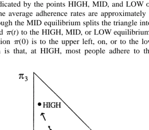
p(t) can be represented on a two-dimensional graph, with p1(t) horizontally, p3(t) vertically, andp2(t) excluded. The relevant region of the graph is the right triangle with unit sides and vertex at the origin. Fig. 1 illustrates. It is like a ‘probability triangle’ from decision theory. The points on and inside the triangle represent the possible values of
p(t). Points to the upper left correspond to higher values of the average adherence rate
f(t)5q9p(t). Given parameters ( q , q , q ) and an initial value1 2 3 p(0), the model generates the path of points p(1), p(2), p(3), . . .
Consider the particular parameter setting ( q , q , q )1 2 3 5(0.06, 0.55, 0.92). It says that a person may be as low as 0.06 likely to obey the norm, as high as 0.92 likely, or at the middle value 0.55. For this setting, computations reveal that there are three equilibria for
p(t), indicated by the points HIGH, MID, and LOW on the figure. At HIGH, MID and LOW, the average adherence rates are approximately 0.83, 0.43, and 0.17. The dashed line through the MID equilibrium splits the triangle into regions of attraction. The model will sendp(t) to the HIGH, MID, or LOW equilibrium depending on whether the initial distribution p(0) is to the upper left, on, or to the lower right of the dashed line. The intuition is that, at HIGH, most people adhere to the norm; hence imitation attracts
people to HIGH. Similarly, at LOW, most people reject the norm; hence imitation attracts people to LOW. The MID equilibrium involves a balance of opposite attractions; hence a push off the dashed line in either direction tips the scale and thus sendsp(t) to either HIGH or LOW. Although the population distribution p(t) thus converges, individuals in the population continue to move among the adherence levels ( q , q , q ),1 2 3
with two important exceptions. If the example had q351 instead of q3,1, then the HIGH equilibrium would be at the upper left corner of the triangle, where everyone would have the single adherence rate q351. Similarly, if the example had q150 instead of q1.0, the LOW equilibrium would be at the lower right corner of the triangle.
Two adjustment paths for p(t) are shown on Fig. 1: a path from p(0)5(0.1, 0.7, 0.2)9 heading toward the HIGH equilibrium, and a path fromp(0)5(0.5, 0.45, 0.05)9
heading toward the LOW equilibrium. Intuitively, Fig. 1 invites us to visualize a ‘turnpike’ running through all three equilibria. For each of the two sample paths shown, the model’s initial movements are as if a search for the turnpike, with repeated, partial overshooting in the process (the initially jagged pattern). Once near the turnpike, the model moves more smoothly along it toward the relevant equilibrium. If the initial point
p(0) were on the dashed line itself, but away from the MID equilibrium, then p(t) would stay on the dashed line, jumping back and forth from one side of MID to the other. Despite the overshooting, the jumps would get smaller, andp(t) would converge to MID.
Fig. 1 suggests fragility in social behavior. Two societies with identical parameters and very similar starting points can display similarly erratic initial behavior, but nonetheless tip to opposite equilibria if their starting points are on opposite sides of the dashed line. A one-time social shock which perturbs a society from the HIGH or LOW equilibrium to the opposite side of the dashed line can tip the society to the opposite equilibrium, with some erratic movement on route. The HIGH or LOW equilibrium is more or less fragile according to whether it is close or far from the dashed line. Further, as discussed below, a perturbation of parameters can change the number of equilibria. Since a central concern of the model is that people may have different degrees of commitment to a norm, the n53 case is not adequate. We think of n as sizable. Thus, we need results for any n$3. The general results to follow can be previewed relative to Fig. 1. So long as q , q , . . . , q have sufficient spread, there will be exactly three1 2 n
equilibria, as on Fig. 1. Further, the regions of attraction for the high and low equilibria will extend all the way to the middle equilibrium, which is thus a tipping point. There will never be more than three equilibria, but there may be two or one. The number of equilibria will be found by counting real roots of an nth degree polynomial.
3. Equilibria and stability
However, for the particular P-matrix (1), we can say much more. In the following theorem and below, a distributionp** will be said to ‘strictly dominate’ a distribution
p*, written p**ssp*, if and only if the cumulative dominance inequalities are all strict:
* ** * * ** **
p . p1 1 ,p 1 p . p1 2 1 1p2 , . . . ,
* * ** **
p 1 ? ? ? 1 p1 n21.p1 1 ? ? ? 1pn21.
Equilibrium theorem. Assume the model (1)–(2), and define an equilibrium to be a
solution p* ofp*5P(p*)9p*.
1. Number of equilibria. The number of equilibria equals the number of distinct real
roots f, in the interval 0#f#1, of the polynomial
n
i21 n2i
p( f )5
O
( f2q )fi (12f ) .i51
That number is one, two, or three. When there is one such root, p9( f ) is positive at
the root. When there are two such roots, p9( f ) is positive at one and zero at the
other. When there are three such roots, p9( f ) is positive at the smallest and largest
roots and negative at the middle root.
2. Benchmark cases. If q150, thenp 5(1, 0, . . . , 0)9is an equilibrium. If qn51, then
p 5(0, . . . , 0, 1)9is an equilibrium. If q150 and qn51, there is a third equilibrium
with all elements ofp positive.
3. Form of an equilibrium. The equilibrium distributionp* corresponding to a root f *
is
1 2 n21 f *
]]]]]]] ]]
p*5
S
2 n21D
(1, x, x , . . . , x )9, where x512f *. 11x1x 1 ? ? ? 1xIf f *51, this equation is taken to mean the limit as f *→1, namelyp*5(0, . . . , 0, 1)9. A root f * and the corresponding p* satisfy f *5q9p*; hence the root is an
equilibrium average adherence probability.
4. Dominance ranking. Multiple equilibria have a strict dominance ranking. That is, if
p* andp** are two equilibria with average adherence probabilities f *5q9p* and
f **5q9p**, then either (i ) p*ssp** and f *.f ** or (ii ) p*aap** and
f *,f **.
In verbal summary: Equilibria correspond to roots of the polynomial p( f ) in the interval 0#f #1; there are one, two, or three; the number is three in the benchmark case when total adherence and total rejection are both possible (when q150 and qn51); each equilibrium p is determined by its root according to the formula in Part 3; and multiple equilibria are dominance ranked. (In addition, the theorem gives information on
Fig. 2. Illustration of three, two, and one root cases.
triple, double, and single equilibrium cases are q5(0.1, 0.4, 0.5, 0.9)9, q5(0.125, 0.5, 0.5, 1.0)9, and q5(0.2, 0.4, 0.5, 0.8)9. Fig. 2, used momentarily in the proof, illustrates the qualitative look of p( f ) in these cases. As Fig. 2 suggests, a double equilibrium involves a tangency root and is thus a knife-edge case; a change in any q will bump thei
tangency up or down, thus eliminating the root or changing it to two roots.The intuition of the three- equilibrium case was discussed in the context of Fig. 1 above. The intuition of other cases can be thought of as perturbations from this case. As we make q larger1
and larger, the low equilibrium will sooner or later be lost because the lowest adherence rates won’t be low enough to support a low equilibrium. Similarly, as we make qn
smaller and smaller, the high equilibrium will be lost.
Proof of the equilibrium theorem. The transition matrix P(p) from (1) depends onp
only through f5q9p. Rewrite P(p) as P( f ) for this paragraph only. Solving the equilibrium conditionp 5P(p)9p for p can be thought of as solvingp 5P( f )9p and
f5q9p simultaneously forp and f. Asterisks, as equilibrium indicators, are suppressed during this proof. The equation p 5P( f )9p can be solved by linear means forp as a function of f, call the solution p 5 a( f ). The ith element is
i 2 n
ai( f )5x / [x1x 1 ? ? ? 1x ], where x5f/(12f ). (3) Combining p 5 a( f ) and f5q9p yields f5q9a( f ) as a scalar equation to solve for equilibrium values of f (subject to 0#f#1). Premultiplying f2q9a( f )50 by
i21 n2i
oi f (12f ) and rearranging yields the polynomial equation p( f )50 from Part 1 of the Equilibrium Theorem. Thus, there is an equilibrium p 5 a( f ) associated with each root of p( f ) in the unit interval. Next show that the number of such roots is one, two, or three. Count roots on the boundary of the unit interval ( f50 or f51) separately from roots in the interior (0,f,1).
Boundary roots. By careful inspection of the polynomial p( f ), f50 is a root if and only if q150, and f51 is a root if and only if qn51. Thus, there may be zero, one, or two boundary roots depending on whether neither, one, or both of the conditions q150 and qn51 hold.
n
Interior roots. Dividing p( f )50 by (12f ) and using the transform x5f/(l2f )
allows p( f )50 to be rewritten
2
12q11(12q12q )x2 1(12q22q )x3 1 ? ? ?
n21 n
by an f in the interval 0,f,1, the number of interior roots of p( f )50 equals the number of positive roots x of (4). That number can be bounded using Descartes’ rule of signs. Moving across the coefficients of (4) from left to right reveals three possible sign changes: (i) a possible sign change from negative to positive between the first two coefficients (12q and 11 2q12q ); (ii) one possible sign change from positive to2
negative among the middle n21 coefficients (12q12q to 12 2qn212q ); and (iii) an
possible sign change from negative to positive between the last two coefficients (12qn212q and 1n 2q ). Regarding (ii), there cannot be more than one sign changen
among the middle n21 coefficients because they are declining in size (since q1#q2# ? ? ? #q ). Thus, three is the maximum number of sign changes. By Descartes’ rule ofn
signs, the number of positive roots x (with multiple roots counted multiply) can be no greater than the number of sign changes. It follows that there are at most three distinct interior roots for f. However, if q150 (and thus f50 is a root), a sign change of type (i) is ruled out. Similarly, if qn51 (and thus f51 is a root), a sign change of type (iii) is ruled out. Therefore, the maximum number of interior roots is three minus the number of boundary roots. That is, the total number of roots cannot exceed three. Numerical examples easily establish that all three possibilities do occur.
To complete proof of Part 1, find the signs of p9( f ) at the roots by considering the graph of p( f ) over 0#f #1, delineating cases. Consider first the case when q1 .0 and
qn,1. Then the graph must be qualitatively as on the illustrations of Fig. 2. To see why, verify from the definition of p( f ) that p(0)5 2q1,0 and p(1)512qn.0. That is, the left end of the graph has negative intercept at f50, and the right end has positive intercept at f51, as illustrated on Fig. 1. But then the only ways to finish the graph with a maximum of three real roots in the unit interval are qualitatively like the cases shown. (Since a tangency intersection always represents a pair of identical roots, two tangency intersections would require more than three roots and thus cannot occur.) The sign claims about p9( f ) then follow. When q150, similar considerations apply, except that the left intersection is at f50. When qn51, the right intersection is at f51.
Part 3 follows immediately from (3) above, and Part 4 follows from Part 3. To verify Part 2, recall from the discussion of boundary roots that the graph of p( f ) has an intersection at f50 when q150 and an intersection at f51 when qn51. The first two sentences of Part 2 then follow from Part 3. To verify the third sentence, first verify that
p9(0).0 and p9(1).0 when q150 and qn51. It follows that the graph of p( f ) must have a third intersection with 0,f,1, and it then follows from Part 3 that, at the corresponding equilibrium, p has all positive elements. h
one of the stable equilibria drops off, leaving one stable and one unstable equilibrium. Part 3 states that, when we move from two to one equilibrium, the unstable equilibrium drops off, leaving one stable equilibrium.
Stability theorem. Distinguish the three main cases:
1. Triple equilibrium. Assume a triple equilibrium (p*,p**,p***) with the dominance
order p*aap**aap***. Then the low equilibrium p* is locally stable, with
region of attraction including every vector strictly dominated by the middle
equilibrium. That is, p(t)→p* if p(0)aap**. Similarly, the high equilibrium in p*** is locally stable, with region of attraction including every vector strictly
dominating the middle equilibrium. That is,p(t)→p*** ifp(0)ssp**. The middle
equilibrium is therefore not locally stable.
2. Double equilibrium. Assume a double equilibrium (p*, p**), with adherence rates ( f *, f **), ordered such that p*aap** and f *,f **. (i ) If p9( f *)50 and
p9( f **).0, thenp* is not locally stable, andp** is locally stable with region of
attraction including every vector strictly dominating p* [that is, p(t)→p** if
p(0)ssp*]. (ii ) In the reverse case, when p9( f *). 0 and p9( f **)50, the reverse
conclusions hold.
3. Single equilibrium. A single equilibrium p* is globally stable; it has region of
attraction including every possible starting point. That is, p(t)→p* for any p(0).
For a triple equilibrium, Part 1 asserts not just local stability for the low and high equilibria, but also regions of attraction extending all the way to the middle, or ‘tipping’, equilibrium. Nonetheless, this is not a complete result. Compare the n53 example of Fig. 1 to Part 1 of the theorem. On Fig. 1, the entire space of p(t) was partitioned into regions of attraction for the three equilibria – above the dashed line, below the dashed line, and the dashed line itself. A corresponding result for the general n$3 case would say that there is a surface in the space ofp(t) such that the regions of attraction for the three equilibria are all initial points to one side of the surface, all to the other side of the surface, and all on the surface itself. We suspect that some such partition exists, but we have not found it. Part 1 is less complete since it does not cover all initial points; rather it covers only points which dominate or are dominated by the middle equilibrium. Nonetheless, proof of the Stability Theorem is long and difficult. See Appendix A. The approach of the proof is to transform the model to terms of the cumulative distribution
4. Conclusion
A spare list of assumptions and a simple parameter set q , q , . . . , q , lead to a variety1 2 n
of more or less fragile equilibrium patterns which seem qualitatively descriptive of the way that real societies ‘tip’ for or against a norm. Imitative influences may lead otherwise identical societies, because of minor differences in initial conditions, to dramatically different equilibria. The equilibria may be robust or fragile. A perturbation of a population distribution – a resetting of initial conditions – may tip a community from one equilibrium to another. A perturbation of parameters may do the same, and more. It may alter the pattern of equilibria, for example by adding a high equilibrium to a society which previously had only a low equilibrium. Relative to other tipping models in the literature, the novelty here is that different people may have different degrees of adherence to a norm, not just all or nothing adherence.
In the case of a triple equilibrium, the model suggests that a temporary perturbation may, by tipping a population from one equilibrium to another, have large and long-lasting effects. Active policy to push a society from norm-rejection to norm-acceptance might be discussed by supposing that the upward step probability f(t) can be increased at a cost. For example, a policy-maker might be able to increase f(t)5q9p(t) to f(t)5
2
s(t)1(12s(t))q9p(t) at a per capita cost of cs(t) , where c is a cost parameter and
s(t) is a policy choice variable obeying 0#s(t)#1. The policy maker’s objective function might be a discounted sum of the adherence rates, net of the discounted sum of costs. The policy problem would be to maximize this objective function subject to the model’s dynamic. Questions are whether intervention is worth the cost, whether intervention should be short and highly intense or more spread out, and so on. The policy-maker might be a government trying to establish a non-smoking norm, a town trying to reestablish some civilized tradition, or an industry trying to establish a new consumer norm.
We have investigated (Conlisk et al., 1999) modifications to the model which allow random variation in the number of steps a person adjusts on the q , q , . . . , q ladder,1 2 n
entry and exit of people from the population, the presence of people who never change adherence rates, and subpopulations (perhaps localities) of people who interact more strongly within subpopulation than between subpopulations. In each of these cases, the existence of locally stable high and low equilibria can still be shown. Other results may be lost; for example, there may be more than three equilibria. These modifications alter the transition matrix P(p), but maintain the convenient dynamic structure p(t11)5
P[p(t)]9p(t). They often alter the fragility of equilibria by expanding or contracting regions of attraction.
Acknowledgements
Appendix A. Proof of Stability Theorem
Restatement of model. First a change of variables. Let P be the cumulative distribution corresponding to p:
P 5(p1,p 1 p1 2, . . . ,p 1 ? ? ? 1 p1 n21)9.
Pis written as an (n21)31 vector because the final cumulative probability is always a one and thus conveys no information. Note that larger elements in P mean lesser adherence to the norm. Thus, asPmoves fromP 5(0, . . . , 0)9toP 5(1, . . . , 1)9, the uncumulated distribution p moves from total adherence p 5(0, . . . , 0, 1)9 to total rejection p 5(1, 0, . . . , 0)9. Dominance relations among equilibria can now be expressed as inequalities. For example, the dominance relation for a triple equilibrium (low, middle, high) isP*4P**4P***. Here and below, ‘4’ between two vectors means that every element of the left vector strictly exceeds the corresponding element of the right vector.
The basic equation of motion p(t11)5P[p(t)]9p(t) can be equivalently restated
P(t 11)5G[P(t)],
where the following definitions apply (with time subscripts suppressed for simplicity).
G(P)5[(12f )J1fJ9]P 1(12f )e, where: (n21)3(n21) matrix with ones along the
J5
F
G
first superdiagonal and zeros elsewhere
(A.1)
e5[(n21)31 vector of the form (0, . . . , 0, 1)9],
f5qn2d 9P,
d 5( q22q , q1 32q , . . . , q2 n2qn21)9.
The expression f5qn2d 9P is an equivalent rewrite of the original definition f5q9p. Note that the vectord is nonnegative.
Jacobian. Differentiation yields the (n21)3(n21) Jacobian matrix =G(P)5
[≠G (i P) /≠Pj]:
=G(P)5(12f )J1fJ9 1[e1(J2J9)P]d 9. (A.2) Since the ith element of e1(J2J9)Pis simply p 1 pi i11,
=G(P)$0 when 0#f#1. (A.3)
That is, the function G(P) is monotone – a help to stability analysis. A second help is:
Lemma. If f * is a root of p( f ) obeying 0#f *#1, if P* is the
corresponding equilibrium, and if l* is the largest eigenvalue
Stability for a triple equilibrium. By Part 1 of the Equilibrium Theorem, the low, middle, and high equilibria occur where p9( f ) is positive, negative, and positive, respectively. Thus, in view of (A.4), the Jacobian ofP(t 11)5G[P(t)] has maximum eigenvalue modulus less than, greater than, and less than one at the three equilibria, respectively. It follows immediately that the three equilibria are locally stable, unstable, and stable, respectively, as claimed. However, the Stability Theorem claims much more. It claims that the stability region of the high equilibrium includes all P-values which strictly dominate the middle equilibrium, and it makes a related claim for the low equilibrium. Since proof for the low equilibrium would closely parallel proof for the high equilibrium, we will prove only the latter.
First define a neighborhood S*** of the high equilibriumP***, where the size of the neighborhood depends on an (n21)31 tolerance vector a:
S***(a)5hPuP**2 P $aj, whereaobeysP**2 P***4a40.
This set includes only vectors which strictly dominate the middle equilibriumP**. The inequalities ona assure that S***(a) includes P***. By pickinga arbitrarily close to the zero vector, we can make S***(a) extend arbitrarily close to the middle equilibrium
P**.
Therefore, to prove the claim in the Stability Theorem, it suffices to prove that, for arbitrarily smalla40, S***(a) is a region of attraction for the high equilibriumP***. However, since the dynamic P(t 11)5G[P(t)] is monotone by (A.3), it suffices to show something simpler. For a monotone dynamic, it suffices to show only that S***(a) is a trapping region; see Theorem 2 of Conlisk (1992). Thus, it suffices to show, for arbitrarily smalla40, thatP(t) in S***(a) impliesP(t 11)5G[P(t)] in S***(a), or equivalently that
P # P**2a ⇒ G(P)# P**2a, for arbitrarily smalla40. (A.5) It remains then to verify (A.5). Start with two preliminary equalities, being sure to distinguish the unrestricted variables ( f,P) from their middle equilibrium values ( f **,
P**)
P**5G(P**)5[(12f **)J1f **J9]P**1(12f **)e,
f2f **5d 9(P**2 P). (A.6)
The first equality of (A.6) notes thatP**, being an equilibrium value, equals G(P**), which in turn equals the right side of the first line. The second equality of (A.6) follows from f5qn2d 9P, which is part of (A.1). Now construct a further identity:
P**2G(P)2a 5[=G(P**)2I]a 1(d 9a)(J9 2J )a 1h[(12f )J1fJ9]1[e2(J9 2J )P**]d 9
Match and cancel terms, using the second equality of (A.6) as needed. The result is 050; hence (A.1) and (A.6) imply (A.7).
Finally, derive (A.5) from (A.7). As noted above,=G(P**) has largest eigenvalue modulus exceeding one. Since=G(P**) is a nonnegative and indecomposable matrix, the eigenvalue, call it l**, is real and greater than one; and l** has a corresponding eigenvector with all elements positive. Leta be this eigenvector; it does not depend on
P. It may be scaled multiplicatively to be as small as desired, thus meeting the ‘arbitrarily small’ condition of (A.5).
Since a is an eigenvector of =G(P**), the first term on the right of (A.7) becomes (l**21)a, which has all elements positive sincel**.1. Further, the premise of (A.5) is that P**2 P 2a is nonnegative; and, for small enough scaling of a, the matrix in braces on the right of (A.7) is nonnegative, regardless of the value of f since the ith element of e2(J9 2J )P** equals the positive number (p 1 pi i11)**. In view of these facts, (A.7) implies
P**2G(P)2a $(l**21)a 1(d 9a)(J9 2J )a,
for appropriately small scaling ofa. Finally, note that the first term on the right of this inequality is first order small in a, whereas the second term is second order small ina. Thus, we may scale a small enough that the right side is nonnegative. (A.5) follows.
Stability for double and single equilibria. When there are two equilibria, Part 1 of the
Equilibrium Theorem states that p9( f ) is zero at one equilibrium and positive at the other. Thus, in view of (A.2), the Jacobian of P(t11)5G[P(t)] has maximum eigenvalue modulus less than one at one equilibrium and equal to one at the other. It follows immediately that the first equilibrium is locally stable. The Stability Theorem claims that the stability region of the first equilibrium extends all the way to the second equilibrium. This can be shown by the same method used in the preceding paragraphs, where the stable and unstable equilibria take the roles of P*** andP**.
Finally, consider the case of a single equilibrium. Since G(P) is monotone, the unique equilibrium must be globally stable; see Theorem 1 of Conlisk (1992).
Proof of Lemma (A.4). First define the (n21)3(n21) matrix B( f ) and the (n21)31 vector b( f ) by
2
12x 2
]]
S D
B( f )5(12f )J1fJ9 and b( f )9 5 n [1, x, x ,? ? ?,xn22], 12x
f
]]
where x5 . 12f
Here b( f ) as it stands is an indeterminate form at f51 / 2 and f51. Therefore, let
b(1 / 2) and b(1) be taken to mean the limits of b( f ) as f→1 / 2 and f→1, namely
b(1 / 2)5(1, 1, . . . , 1, 1)9 and b(1)5(0, 0, . . . , 0, 1)9. It can be shown that, at an equilibrium value f * of f with corresponding equilibrium distribution P*,
b( f *)5e2(J9 2J )P* and =G(P*)5B( f *)1b( f *)d 9,
Theorem, the ith element of the left side is also (p 1 pi i11)*. The second equality then follows from (A.2).
Keeping in mind that, in (A.4), all functions of f are evaluated at a solution f * of
p( f )50, simplify notation by writing f *,=G(P*), B( f *), b( f *), andl* as simply f,
B is nonnegative and, with 0,f,1, is indecomposable. By a standard matrix theorem, the dominant eigenvalue of B is a real number lying strictly between the minimum and maximum column sums of B, which are ( f, 1, . . . , 1, 12f ). Thus, the dominant
eigenvalue of B is less than one. It follows that I2B is nonsingular with series inverse
21 2 21
(I2B ) 5I1B1B 1 ? ? ? and that (I2B ) b5b1(nonnegative terms). Since
21
b40 (given 0,f,1), then (I2B ) b40.
The following equation is a definitional identity. To verify it, replace =G by
=G5B1bd 9 (from five paragraphs above), replace b by the definition given, and match terms.
Rephrase this implication as follows. If b .1, there exists an (n21)31 vector a,
21
namely a 5(I2B ) b, such that =Ga4a40, where a40 follows from (A.8). But, by standard nonnegative matrix theory,=Ga4a40 is necessary and sufficient for =G to have dominant eigenvalue strictly greater than one. Thus, we know that
b .1 ⇒ l .1. By parallel reasoning, the two further implications b 51 ⇒ l 51
21 21
three steps: Evaluate (I2B ) ; evaluateb 5 d 9(I2B ) b; and then verify (A.10). This
is a large chore. A large number of algebraic details are elided in the following.
21
Step 1. Evaluate (I2B ) . Again use the transform x5f/(12f ), which is positive
since 0,f,1. Distinguish two subcases.
Case (i). f±1 / 2 and thus x±1. Let u (for unit) denote the (n21)31 vector with all
elements equal to one; let U (for upper) denote the upper triangular matrix with all elements on or below the diagonal equal to zero and with all elements above the diagonal equal to one; and let D be the (n21)3(n21) diagonal matrix D5diag (x,
So only the first i21 elements ofui are nonzero. The inverse expression from Step 1
21
plus substantial manipulation yields the ith element ofd 9(I2B ) :
21 In view of the definition of b5b( f ), manipulations using (A.11) yield
21
Substituting (A.13) in (A.12) and simplifying yields the needed expression for b 5
21
21 closely related task of finding h9(x), evaluated at a root of h(x)50, where h(x) is the nth degree polynomial on the left of Eq. (4). Differentiation and substantial manipulation yield
Eliminating u9DNq between (A.14) and (A.17) yields, after substantial manipulation,
2
Arthur, W.B., 1988. Self-reinforcing mechanisms in economics. In: Anderson, P.W., Arrow, K.J., Pines, D. (Eds.), The Economy as an Evolving Complex System. Addison-Wesley, Redwood City, CA, pp. 9–31. Arthur, W.B., 1989. Increasing returns, competing technologies and lock-in by historical small events: the
dynamics of allocation under increasing returns to scale. Economic Journal 99, 116–131.
Banerjee, A.V., 1992. A simple model of herd behavior. Quarterly Journal of Economics 107, 797–817. Bartholomew, D.J., 1982. Stochastic Models for Social Processes, 3rd Edition. Wiley, New York. Bicchieri, C., Jeffrey, R., Skyrms, B. (Eds.), 1997. The Dynamics of Norms. Cambridge University Press. Bikhchandani, S., Hirshleifer, D., Welch, I., 1992. A theory of fads, fashion, custom, and cultural change as
Bowles, S., 1998a. Endogenous preferences: the cultural consequences of markets and other economic institutions. Journal of Economic Literature 36, 75–111.
Bowles, S., 1998b. Mandeville’s mistake: the evolution of norms in market environments. Manuscript, Department of Economics, University of Massachusetts at Amherst.
Bowles, S., Gintis, H., 1998. The moral economy of communities: structured populations and the evolution of pro-social norms. Evolution and Human Behavior 19, 3–25.
Boyd, R., Richerson, P.J., 1985. Culture and the Evolutionary Process. University of Chicago Press, Chicago. Brock, W., Durlauf, S., 1995. Discrete choice with social interactions I: theory. Santa Fe Institute Working
Paper 95-10-084.
Conlisk, J., 1992. Stability and monotonicity for interactive Markov chains. Journal of Mathematical Sociology 17, 127–143.
Conlisk, J., Gong, J.-C., Tong, C., 1999. Dynamics of imitation and uniformity. Journal of Mathematical Sociology, forthcoming.
Ellison, G., Fudenberg, D., 1995. Word of mouth communication and social learning. Quarterly Journal of Economics 110, 93–125.
Elster, J., 1989a. The Cement of Society. Cambridge University Press, Cambridge.
Elster, J., 1989b. Social norms and economic theory. Journal of Economic Perspectives 3, 99–117. Granovetter, M., 1978. Threshold models of collective behavior. American Journal of Sociology 83,
1420–1443.
Granovetter, M., Soong, R., 1986. Threshold models of interpersonal effects in consumer demand. Journal of Economic Behavior and Organization 7, 83–99.
Kirman, A., 1993. Ants, rationality, and recruitment. Quarterly Journal of Economics 108, 137–156. Ross, L., Nisbett, R.E., 1991. The Person and the Situation. Temple University Press, Philadelphia. Schelling, T.C., 1978. Micromotives and Macrobehavior. Norton, London.
Smallwood, D., Conlisk, J., 1979. Product quality in markets where consumers are imperfectly informed. Quarterly Journal of Economics 93, 1–23.
Weibull, J., 1995. Evolutionary Game Theory. MIT Press, Cambridge, MA. Young, H.P., 1993. The evolution of conventions. Econometrica 61, 57–84.