arXiv:1709.05981v1 [hep-lat] 15 Sep 2017
Breaking in QCD
Hideo Suganuma
Department of Physics, Kyoto University, Kyoto 606-8502, Japan
Takahiro M. Doi
Theoretical Research Division, Nishina Center, RIKEN, Saitama 351-0198, Japan
Krzysztof Redlich, Chihiro Sasaki
Institute of Theoretical Physics, University of Wroclaw, PL-50204 Wroclaw, Poland
Augst 2017
Abstract. We study the relation between quark confinement and chiral symmetry breaking in QCD. Using lattice QCD formalism, we analytically express the various “confinement indicators”, such as the Polyakov loop, its fluctuations, the Wilson loop, the inter-quark potential and the string tension, in terms of the Dirac eigenmodes. In the Dirac spectral representation, there appears a power of the Dirac eigenvalueλnsuch as λNt−1
n , which behaves as a reduction factor for smallλn. Consequently, since this
reduction factor cannot be cancelled, the low-lying Dirac eigenmodes give negligibly small contribution to the confinement quantities, while they are essential for chiral symmetry breaking. These relations indicate no direct, one-to-one correspondence between confinement and chiral symmetry breaking in QCD. In other words, there is some independence of quark confinement from chiral symmetry breaking, which can generally lead to different transition temperatures/densities for deconfinement and chiral restoration. We also investigate the Polyakov loop in terms of the eigenmodes of the Wilson, the clover and the domain-wall fermion kernels, respectively, and find the similar results. The independence of quark confinement from chiral symmetry breaking seems to be natural, because confinement is realized independently of quark masses and heavy quarks are also confined even without the chiral symmetry.
1. Introduction
the description of high-energy hadron reactions in the framework of the parton model [5, 6, 7].
In the low-energy region, however, QCD is a fairly difficult theory because of its strong-coupling nature, and shows nonperturbative properties such as color confinement and spontaneous chiral-symmetry breaking [8, 9]. Here, spontaneous symmetry breaking appears in various physical phenomena, whereas the confinement is highly nontrivial and is never observed in most fields of physics.
For such nonperturbative phenomena, lattice QCD formalism was developed as a robust approach based on QCD [10, 11], and M. Creutz first performed lattice QCD Monte Carlo calculations around 1980 [12]. Owing to lots of lattice QCD studies [13] so far, many nonperturbative aspects of QCD have been clarified to some extent. Nevertheless, most of nonperturbative QCD is not well understood still now.
In particular, the relation between quark confinement and spontaneous chiral-symmetry breaking is not clear, and this issue has been an important difficult problem in QCD for a long time. A strong correlation between confinement and chiral symmetry breaking has been suggested by approximate coincidence between deconfinement and chiral-restoration temperatures [13, 14], although it is not clear whether this coincidence is quantitatively precise or not. At the physical point of the quark massesmu,dandms, a lattice QCD work [15] shows about 25MeV difference between deconfinement and chiral-restoration temperatures, i.e.,Tdeconf ≃176MeV andTchiral ≃151MeV, whereas a recent
lattice QCD study [16] shows almost the same transition temperatures ofTdeconf ≃Tchiral,
after solving the scheme dependence of the Polyakov loop.
The correlation of quark confinement with chiral symmetry breaking is also suggested in terms of QCD-monopoles [17, 18, 19], which topologically appear in QCD in the maximally Abelian gauge. These two nonperturbative phenomena simultaneously lost by removing the QCD-monopoles from the QCD vacuum generated in lattice QCD [18, 19]. This lattice QCD result surely indicates an important role of QCD-monopoles to confinement and chiral symmetry breaking, and they could have some relation through the monopole, but their direct relation is still unclear.
As an interesting example, a recent lattice study of SU(2)-color QCD with Nf = 2 exhibits that a confined but chiral-restored phase is realized at a large baryon density [20]. We also note that a large difference between confinement and chiral symmetry breaking actually appears in some QCD-like theories as follows:
• In an SU(3) gauge theory with adjoint-color fermions, the chiral transition occurs at much higher temperature than deconfinement, Tchiral≃8 Tdeconf [21].
• In 1+1 QCD with Nf ≥ 2, confinement is realized, whereas spontaneous chiral-symmetry breaking never occur, because of the Coleman-Mermin-Wagner theorem.
• In N = 1 SUSY 1+3 QCD with Nf =Nc+ 1, while confinement is realized, chiral symmetry breaking does not occur.
have been done so far [17, 18, 19, 22, 23, 24, 25, 26, 27, 28, 29].
One of the key points to deal with chiral symmetry breaking is low-lying Dirac eigenmodes, since Banks and Casher discovered that these modes play the essential role to chiral symmetry breaking in 1980 [9]. In this paper, keeping in mind the essential role of low-lying Dirac modes to chiral symmetry breaking, we deriveanalytical relations
[26, 27, 28, 29] between the Dirac modes and the “confinement indicators”, such as the Polyakov loop, the Polyakov-loop fluctuations [30, 31], the Wilson loop, the inter-quark potential and the string tension, in lattice QCD formalism. Through the analyses of these relations, we investigate the correspondence between confinement and chiral symmetry breaking in QCD.
The organization of this paper is as follows. In Sec. 2, we briefly review the Dirac operator, and its eigenvalues and eigenmodes in lattice QCD. In Sec. 3, we derive an analytical relation between the Polyakov loop and Dirac modes in temporally odd-number lattice QCD, and show independence of quark confinement from chiral symmetry breaking. In Sec. 4, we investigate deconfinement and chiral restoration in finite temperature QCD, through the relation of the Polyakov-loop fluctuations with Dirac eigenmodes. In Sec. 5, we derive analytical relations of the Polyakov loop with Wilson, clover and domain wall fermions, respectively. In Sec. 6, we express the Wilson loop with Dirac modes on arbitrary square lattices, and investigate the string tension, quark confining force, in terms of chiral symmetry breaking. Section 7 is devoted to summary and conclusion.
Through this paper, we take normal temporal (anti-)periodicity for gauge and fermion variables, i.e., gluons and quarks, as is necessary to describe the thermal system properly, on an ordinary square lattice with the spacing a and the size V ≡ N3
s ×Nt. For the simple notation, we mainly use the lattice unit of a= 1, although we explicitly writeaas necessary. The numerical calculation is done in SU(3) quenched lattice QCD.
2. Dirac operator, Dirac eigenvalues and Dirac modes in lattice QCD
In this section, we briefly review the Dirac operator ˆD6 , Dirac eigenvalues λn and Dirac modes |ni in lattice QCD, where the gauge variable is described by the link-variable Uµ(s) ≡ eiagAµ(s) ∈ SU(Nc) with the gauge coupling g and the gluon field Aµ(x)∈su(Nc).
For the simple notation, we useU−µ(s)≡Uµ†(s−µˆ), and introduce the link-variable operator ˆU±µ defined by the matrix element [25, 26, 27, 28]
hs|Uˆ±µ|s′i=U±µ(s)δs±µ,sˆ ′, (1) which satisfies ˆU−µ= ˆUµ†. In lattice QCD formalism, the simple Dirac operator and the covariant derivative operator are given by
ˆ
6
D= 1
2a
4
X
µ=1
γµ( ˆUµ−Uˆ−µ), Dˆµ = 1
The Dirac operator ˆD6 is anti-hermite satisfying ˆ
6
D†s′,s =−D6ˆs,s′, (3)
so that its eigenvalue is pure imaginary. We define the normalized Dirac eigenmode |ni
and the Dirac eigenvalue λn, ˆ
6
D|ni=iλn|ni (λn ∈R), hm|ni=δmn. (4)
Since the eigenmode of any (anti)hermite operator generally makes a complete set, the Dirac eigenmode |ni of anti-hermite ˆD6 satisfies the complete-set relation,
X
and its explicit form is given by 1
For the thermal system, considering the temporal anti-periodicity in ˆD4 acting on
quarks [32], it is convenient to add a minus sign to the matrix element of the temporal link-variable operator ˆU±4 at the temporal boundary oft =Nt as [28]
hs, Nt|Uˆ4|s,1i = −U4(s, Nt),
hs,1|Uˆ−4|s, Nti= −U−4(s,1) = −U4†(s, Nt), (8) which keeps ˆU−µ = ˆUµ†. The standard Polyakov loop LP defined with U4(s) is simply
written as the functional trace of ˆUNt
4 ,
with the four-dimensional lattice volumeV ≡N3
s×Nt, the functional trace Trc ≡Pstrc, and the trace trc over color index. The minus sign stems from the additional minus on U4(s, Nt), which reflects the temporal anti-periodicity ofD6 [28, 32].
We here comment on the gauge ensemble average and the functional trace of operators in lattice QCD. In the numerical calculation process of lattice QCD, one first generates many gauge configurations by importance sampling with the Monte Carlo method, and next evaluates the expectation value of the operator in consideration at each gauge configuration, and finally takes its gauge ensemble average. In lattice QCD, the functional trace is expressed by a sum over all the space-time site, i.e., Tr = P
str, which is defined for each lattice gauge configuration. On enough large volume lattice, e.g.,Ns → ∞, the functional trace is proportional to the gauge ensemble average, Tr ˆO = P
definition of ˆU±µin Eq.(1), the functional trace of any product of link-variable operators corresponding to “non-closed line” is exactly zero, i.e.,
Tr(
at each lattice gauge configuration [26, 27, 28], before taking the gauge ensemble average. To finalize in this section, we briefly introduce the crucial role of low-lying Dirac modes to chiral symmetry breaking. For each gauge configuration, the Dirac eigenvalue distribution is defined by
and then the Dirac zero-eigenvalue densityρ(0) relates to the chiral condensate hqq¯ ivia the Banks-Casher relation [9]
|hqq¯ i|= lim
m→0Vlim→∞πρ(0). (12)
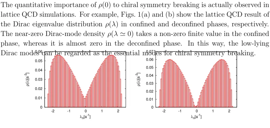
The quantitative importance ofρ(0) to chiral symmetry breaking is actually observed in lattice QCD simulations. For example, Figs. 1(a) and (b) show the lattice QCD result of the Dirac eigenvalue distribution ρ(λ) in confined and deconfined phases, respectively. The near-zero Dirac-mode densityρ(λ≃0) takes a non-zero finite value in the confined phase, whereas it is almost zero in the deconfined phase. In this way, the low-lying Dirac modes can be regarded as the essential modes for chiral symmetry breaking.
0
Figure 1. The lattice QCD result of the Dirac eigenvalue distribution ρ(λ) in the lattice unit for (a) the confinement phase (β= 5.6, 103×5) and (b) the deconfinement
phase (β= 6.0, 103×5). This figure is taken from Ref. [27].
3. Polyakov loop and Dirac modes in temporally odd-number lattice QCD
In this section, we study the Polyakov loop and Dirac modes in temporally odd-number lattice QCD [26, 27, 28], where the temporal lattice size Nt(< Ns) is odd. Note that, in the continuum limit ofa →0 with keeping Nta constant, any large number Nt gives the same physical result. Then, it is no problem to use the odd-number lattice.
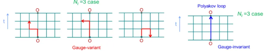
Figure 2. (a) A simple example of the temporally odd-number lattice (Nt= 3 case). (b) Only gauge-invariant quantities such as closed loops and the Polyakov loop survive in QCD. Closed loops have even-number links on the square lattice.
3.1. Analytical relation between Polyakov loop and Dirac modes
On the temporally odd-number lattice, we consider the functional trace [26, 27, 28],
I ≡Trc,γ( ˆU4D6ˆ
Nt−1
), (13)
where Trc,γ ≡ Pstrctrγ includes the sum over all the four-dimensional site s and the traces over color and spinor indices. From Eq.(2), ˆU4D6ˆ
Nt−1
is written as a sum of products of Nt link-variable operators, since the lattice Dirac operator ˆD6 includes one link-variable operator ˆU in each direction of ±µ. Then, ˆU4D6ˆ
Nt−1
is expressed as a sum of many Wilson lines with the total length Nt, as shown in Fig.3.
Figure 3. Examples of the trajectories stemming fromI= Trc,γ( ˆU4D6ˆ
Nt−1
). For each trajectory, the total length isNt, and the “first step” is positive temporal direction corresponding to ˆU4. All the trajectories with the odd-number length Nt cannot
form a closed loop on the square lattice, so that they are gauge-variant and give no contribution, except for the Polyakov loop.
Note that all the trajectories with the odd-number length Nt cannot form a closed loop on the square lattice, and corresponding Wilson lines are gauge-variant, except for the Polyakov loop. In fact, almost all the trajectories stemming fromI = Trc,γ( ˆU4D6ˆ
Nt−1
) is non-closed and give no contribution, whereas only the Polyakov-loop component in I can survive as a gauge-invariant quantity. Thus,I is proportional to the Polyakov loop LP. Actually, using Eqs.(9) and (10), one can mathematically derive the relation of
I = Trc,γ( ˆU4D6ˆ
Nt−1
= 4
where the last minus reflects the temporal anti-periodicity of ˆD6 [28, 32]. On the other hand, using the completeness of the Dirac mode, P
n|nihn| = 1, we calculate the functional trace in Eq.(13) and find the Dirac-mode representation of
I =X
Combing Eqs.(14) and (15), we obtain the analytical relation between the Polyakov loopLP and the Dirac modes in QCD on the temporally odd-number lattice [26, 27, 28],
LP =−
which is mathematically robust in both confined and deconfined phases. From Eq.(16), one can investigate each Dirac-mode contribution to the Polyakov loop individually.
Using the Dirac eigenvalue distribution ρ(λ)≡ V1 P
As a remarkable fact, because of the strong reduction factorλNt−1
n , low-lying Dirac-mode contribution is negligibly small in RHS of Eq.(16). In Eq.(17), the reduction factor λNt−1 cannot be cancelled by other factors, because ρ(0) is finite (not divergent) as the
Banks-Casher relation suggests, and U4(λ) is also finite reflecting the compactness of
U4 ∈SU(Nc).
To conclude, the low-lying Dirac modes give little contribution to the Polyakov loop, regardless of confined or deconfined phase [26, 27, 28].
3.2. Properties on analytical relation between Polyakov loop and Dirac modes
In order to emphasize the importance and generality of Eq.(16), we summarize its essential properties;
(i) The relation (16) is manifestly gauge invariant, because of the gauge invariance of
hn|Uˆ4|ni=Pshn|sihs|Uˆ4|s+ ˆtihs+ ˆt|ni=Psψn†(s)U4(s)ψn(s+ ˆt) under the gauge transformation, ψn(s)→V(s)ψn(s).
(ii) In RHS, there is no cancellation between chiral-pair Dirac eigen-states, |ni and γ5|ni, since (Nt−1) is even, i.e., (−λn)Nt−1 =λNnt−1, andhn|γ5Uˆ4γ5|ni=hn|Uˆ4|ni.
(iii) The relation (16) is valid in a large class of gauge group of the theory, including SU(Nc) gauge theory with any color number Nc.
(iv) The relation (16) is also intact regardless of presence or absence of dynamical quarks, although dynamical-quark effects appear in LP, the Dirac eigenvalue distribution ρ(λ) and hn|Uˆ4|ni. Equation (16) remains valid at finite density and
Note here that Eq.(16) has the above-mentioned generality and wide applicability, because our derivation is based on only a few setup conditions [28]:
1. square lattice (including anisotropic cases) with temporal periodicity 2. odd-number temporal size Nt(< Ns)
In the following, we reconsider the technical merit to use the temporally odd-number lattice, i.e., absence of the loop contribution, by comparing with even-number lattices. When Nt is even, a similar argument can be applied through the relations
I′ ≡ Trc,γ(γ4Uˆ4D6ˆ
Nt−1
) =X n
hn|γ4Uˆ4D6ˆ
Nt−1
|ni
=iNt−1X n
λNt−1
n hn|γ4Uˆ4|ni, (18)
however, apart from the Polyakov loop, there remains additional contribution from huge number of various loops (including reciprocating line-like trajectories) as
I′ ≡ Trc,γ(γ4Uˆ4D6ˆ
Nt−1
) = 1
2Nt−1 Trc,γ[γ4
ˆ U4{
4
X
µ=1
γµ( ˆUµ−Uˆ−µ)}Nt−1]
= −4NcV
2Nt−1LP + (loop contribution), (19)
and thus one finds
LP =−
(2i)Nt−1
4NcV X
n
λNt−1
n hn|γ4Uˆ4|ni+ (loop contribution), (20)
where the relation between the Polyakov loop LP and Dirac modes is not at all clear, owing to the complicated loop contribution. In the continuum limit, both equations (16) and (20) simultaneously hold, and there appears some constraint on the loop contribution, which is not of interest. In fact, by the use of the temporally odd-number lattice, all the additional loop contributions disappear, and one gets a transparent correspondence as Eq.(16) between the Polyakov loop and Dirac modes. (For the other type of the formula on even-number lattices, see Appendix A in Ref.[26].)
3.3. Numerical analysis of the low-lying Dirac-mode contribution to the Polyakov loop
Now, we perform lattice QCD Monte Carlo calculations on the temporally odd-number lattice, and investigate the relation (16) and the low-lying Dirac-mode contribution to the Polyakov loop.
To begin with, we calculate LHS and RHS in Eq.(16) independently, and compare these values in both confined and deconfined phases [26, 27]. The Polyakov loop LP, i.e., the LHS, can be calculated in lattice QCD straightforwardly, following the definition in Eq.(9). For RHS in Eq.(16), we numerically solve the eigenvalue equation (7), and get all the eigenvalues λn and the eigenfunctions ψn(s). Once the Dirac eigenfunction ψn(s) is obtained, the matrix element hn|Uˆ4|ni can be calculated as
As a numerical demonstration of Eq.(16), we calculate its LHS (LP) and RHS (Dirac spectral sum) for each gauge configuration generated in quenched SU(3) lattice QCD, and show representative values in confined and deconfined phases in Tables 1 and 2, respectively. In both phases, one finds the exact relation LP = RHS in Eq.(16) at each gauge configuration. [Even in full QCD, the mathematical relation (16) must be valid, which is to be numerically confirmed in our future study.]
Table 1. Numerical lattice-QCD results for LHS (LP) and RHS (Dirac spectral sum) of the relation (16) in the confinement phase with β = 5.6 on 103×5 size lattice for
each gauge configuration (labeled with “Config. No.”) We also list (LP)IR-cutwith the
IR Dirac-mode cutoff of ΛIR≃0.4GeV. This data is partially taken from Ref. [26].
Config. No. 1 2 3 4 5 6 7
ReLP 0.00961 -0.00161 0.0139 -0.00324 0.000689 0.00423 -0.00807 Re RHS 0.00961 -0.00161 0.0139 -0.00324 0.000689 -0.00423 -0.00807 Re(LP)IR-cut 0.00961 -0.00160 0.0139 -0.00325 0.000706 0.00422 -0.00807
ImLP -0.00322 -0.00125 -0.00438 -0.00519 -0.0101 -0.0168 -0.00265 Im RHS -0.00322 -0.00125 -0.00438 -0.00519 -0.0101 -0.0168 -0.00265 Im(LP)IR-cut -0.00321 -0.00125 -0.00437 -0.00520 -0.0101 -0.0168 -0.00264
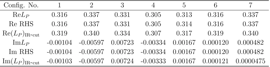
Table 2. Numerical lattice-QCD results for LHS (LP) and RHS (Dirac spectral sum) of the relation (16) in the deconfinement phase withβ = 5.7 on 103×3 size lattice for
each gauge configuration (labeled with “Config. No.”) We also list (LP)IR-cutwith the
IR Dirac-mode cutoff of ΛIR≃0.4GeV. This data is partially taken from Ref. [26].
Config. No. 1 2 3 4 5 6 7
ReLP 0.316 0.337 0.331 0.305 0.313 0.316 0.337 Re RHS 0.316 0.337 0.331 0.305 0.314 0.316 0.337 Re(LP)IR-cut 0.319 0.340 0.334 0.307 0.317 0.319 0.340
ImLP -0.00104 -0.00597 0.00723 -0.00334 0.00167 0.000120 0.000482 Im RHS -0.00104 -0.00597 0.00723 -0.00334 0.00167 0.000120 0.000482 Im(LP)IR-cut -0.00103 -0.00597 0.00724 -0.00333 0.00167 0.000121 0.0000475
Next, we introduce the IR cutoff of ΛIR ≃0.4GeV for the Dirac modes, and remove
the low-lying Dirac-mode contribution for |λn|<ΛIR from RHS in Eq.(16). The chiral
condensate after the removal of IR Dirac-modes below ΛIR is expressed as
hqq¯ iΛIR =− 1 V
X
|λn|≥ΛIR
2m λ2
n+m2q
. (21)
In the confined phase, this IR Dirac-mode cut leads to hqq¯iΛIR
hqq¯i ≃0.02 and almost
chiral-symmetry restoration in the case of physical current-quark mass, mq ≃5MeV [26]. We calculate (LP)IR-cut with the IR Dirac-mode cutoff of ΛIR ≃0.4GeV, and add
One finds that LP ≃(LP)IR-cut is satisfied for each gauge configuration in both phases.
For the configuration average, hLPi ≃ h(LP)IR-cuti is of course satisfied.
From the analytical relation (16) and the numerical lattice QCD calculation, we conclude that low-lying Dirac-modes give negligibly small contribution to the Polyakov loop LP, and are not essential for confinement, while these modes are essential for chiral symmetry breaking. This indicates no direct one-to-one correspondence between confinement and chiral symmetry breaking in QCD.
4. Role of Low-lying Dirac modes to Polyakov-loop fluctuations
In thermal QCD, the Polyakov loop has fluctuations in longitudinal and transverse directions, as shown in Fig.4(a), and the Polyakov-loop fluctuation gives a possible indicator of deconfinement transition [30, 31]. In this section, we investigate the Polyakov-loop fluctuations and the role of low-lying Dirac modes [27] in the deconfinement transition at finite temperatures.
For the Polyakov loop LP, we define its longitudinal and transverse components,
LL≡Re ˜LP, LT ≡Im ˜LP, (22)
with ˜LP ≡LP e2πik/3wherek ∈ {0,±1}is chosen such that theZ3-transformed Polyakov
loop lies in its real sector [27, 30, 31]. We introduce the Polyakov-loop fluctuations as
χA∝ h|LP|2i − |hLPi|2, χL∝ hL2Li − hLLi2, χT ∝ hL2Ti − hLTi2, (23) and consider their different ratios which are known to largely change around the transition temperature [30, 31], thus can be used as a good indicator of the deconfinement transition.
As an illustration, we show in Fig.4(b) the temperature dependence of the ratio RA ≡χA/χL. Around the transition temperature, one finds a large change ofRAon the Polyakov-loop fluctuation, which reflects the onset of deconfinement, while the rapid reduction of the chiral condensate indicates a signal of chiral symmetry restoration. As a merit to use the ratio RA instead of the individual fluctuations, multiplicative-type uncertainties related to the renormalization of the Polyakov loop are expected to be cancelled to a large extent in the ratio.
Similarly in Sec. 3, we derive Dirac-mode expansion formulae for Polyakov-loop fluctuations in temporally odd-number lattice QCD [27]. For the ratios RA ≡ χA/χL and RT ≡χT/χL, we obtain their Dirac spectral representation as
Figure 4. (a) The scatter plot of the Polyakov loop in lattice QCD. The original figure is taken from Ref.[33]. (b) The temperature dependence of the Polyakov loop susceptibilities ratioRA ≡χA/χL and the light-quark chiral condensatehψψ¯ il,
normalized to its zero temperature value on a finite lattice. The lattice QCD Monte Carlo data are from Refs. [31] and [34], respectively. This figure is taken from Ref.[27].
with ˆUnn
4 ≡ hn|Uˆ4|ni. We note that all the Polyakov-loop fluctuations are almost
unchanged by removing low-lying Dirac modes [27] in both confined and deconfined phases, because of the significant reduction factor λNt−1
n appearing in the Dirac-mode sum.
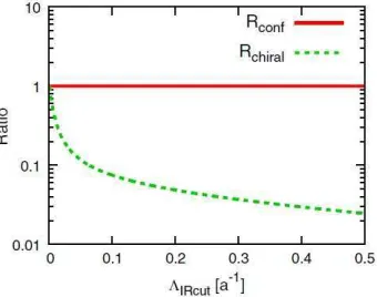
Next, let us consider the actual removal of low-lying Dirac-mode contribution from the Polyakov-loop fluctuation using Eqs.(24) and (25), and also the chiral condensate for comparison. As an example, we show in Fig.5 the lattice QCD result of
Rconf(ΛIRcut)≡
RA(ΛIRcut)
RA
, Rchiral(ΛIRcut)≡
hqq¯ iΛIRcut
hqq¯ i (26)
in the presence of the infrared Dirac-mode cutoff ΛIRcut in the confined phase (β = 5.6,
103×5) [27]. Here, R
A(ΛIRcut) denotes the truncated value of RA when the low-lying Dirac-mode contribution of |λn| < ΛIRcut is removed from the Dirac spectral sum in
Eq.(24). The truncated chiral condensate hqq¯ iΛIRcut is defined with Eq.(21), and the current-quark mass is taken as mq=5MeV.
In contrast to the strong sensitivity of the chiral condensate Rchiral(ΛIRcut), the
Polyakov-loop fluctuation ratio Rconf(ΛIRcut) is almost unchanged against the infrared
cutoff ΛIRcut of the Dirac mode [27], as discussed after Eq.(25). Thus, we find no
significant role of low-lying Dirac modes for the Polyakov-loop fluctuation as a new-type confinement/deconfinement indicator, which also indicates independence of confinement from chiral property in thermal QCD.
5. Relations of Polyakov loop with Wilson, clover and domain wall fermions
Figure 5. The lattice QCD result of IR Dirac-mode-removed quantities of
Rconf(ΛIRcut)≡RA(ΛIRcut)/RAandRchiral(ΛIRcut)≡ hqq¯ iΛIRcut/hqq¯ iformq= 5 MeV,
plotted against the infrared cutoff ΛIRcutintroduced on Dirac eigenvalues, in quenched
lattice withβ = 5.6 and 103×5 (confined phase). This figure is taken from Ref.[27].
the mathematical eigenfunction of ˆD6 .
However, one may wonder the doublers [13] in the use of the lattice Dirac operator ˆ
6
D in Eq.(2), although it is not the problem in the above formulae. In fact, according to the Nielsen-Ninomiya theorem [35], 2d modes simultaneously appear per fermion on a lattice, if one uses a bilinear fermion action satisfying translational invariance, chiral symmetry, hermiticity and locality, on a d-dimensional lattice. Then, for the description of hadrons without the redundant doublers, one adopts Wilson, staggered, clover, domain-wall (DW) or overlap fermion [13, 36, 37, 38, 39, 40], and has to deal with the fermion kernel K, which is more complicated than the simple Dirac operator
ˆ
6
D. In fact, the realization of a chiral fermion on a lattice is not unique. However, in the continuum limit, they must lead to the same physical result. Consequently, it is meaningful to examine our formulation with various fermion actions to get the robust physical conclusion.
In this section, we express the Polyakov loop with the eigenmodes of the kernel of the Wilson fermion, the clover (O(a)-improved Wilson) fermion and the DW fermion [29]. (The formulation with the overlap fermion is found in Ref. [41].)
5.1. The Wilson fermion
A simple way to remove the redundant fermion doublers is to make their mass extremely large by an additional interaction. The Wilson fermion is constructed on a four-dimensional lattice by adding the O(a) Wilson term [13], which explicitly breaks the chiral symmetry. For the Wilson fermion, all the doublers acquire a large mass ofO(a−1)
The Wilson fermion kernel is described with the link-variable operator ˆU±µ as [29]
ˆ
K = ˆD6 +m+ r
2a
±4
X
µ=±1
γµ( ˆUµ−1)
= 1 2a
4
X
µ=1
γµ( ˆUµ−Uˆ−µ) +m+ r 2a
4
X
µ=1
γµ( ˆUµ+ ˆU−µ−2), (27)
which goes to ˆK ≃( ˆD6 +m) +arDˆ2 near the continuum, a≃0. Thus, the Wilson term
arDˆ2 is O(a). The Wilson parameter r is real. Note that each term of ˆK includes one
ˆ
U±µ at most, and connects only the neighboring site or acts on the same site.
For the Wilson fermion kernel ˆK, we define its eigenmode |nii and eigenvalue ˜λn, ˆ
K|nii=iλ˜n|nii, λ˜n∈C. (28)
If the Wilson term is absent, the eigenmode of ˆK = ˆD6 +m is given by the simple Dirac eigenmode|ni, i.e., ˆK|ni= (iλn+m)|ni, and satisfies the completeness ofPn|nihn|= 1. In the presence of the O(a) Wilson term, ˆK is neither hermite nor anti-hermite, and the completeness generally includes an O(a) error,
X
n
|niihhn|= 1 +O(a). (29)
Here, we consider the functional trace J on a lattice withNt= 4l+ 1 (l = 1,2, ...),
J ≡Tr( ˆU42l+1Kˆ2l). (30) By the use of the quasi-completeness (29) for |nii, one finds, apart from an O(a) error,
J ≃X
n
hhn|Uˆ42l+1Kˆ2l|nii=X n
(i˜λn)2lhhn|Uˆ42l+1|nii. (31)
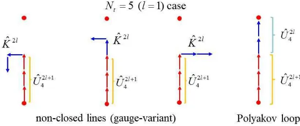
Since the kernel ˆK in Eq. (27) is a first-order equation of the link-variable operator ˆU, J ≡ Tr( ˆU42l+1Kˆ2l) is expressed as a sum of products of ˆU with some c-number factor.
In each product in J, the total number of ˆU does not exceed Nt= 4l+ 1, because ˆK is a first-order equation of ˆU. Each product gives a trajectory as shown in Fig.6.
Figure 6. Some examples of the trajectories (corresponding to products of ˆU) in
J≡Tr( ˆU2l+1
4 Kˆ2l) for theNt= 5 (l= 1) case. The length does not exceedNtfor each
Among these many trajectories, only the Polyakov loopLP can form a closed loop and
Using the eigenvalue distribution ρ(˜λ)≡ 1
V
by other factors, because of the finiteness of ρ(0) andu(˜λ) reflecting the Banks-Casher relation and the compactness of U4 ∈ SU(Nc). Thus, owing to the strong reduction factor ˜λ2l
n on the eigenvalue ˜λn of the Wilson fermion kernel ˆK, we find also small contribution from low-lying modes of ˆK toLP.
5.2. The clover (O(a)-improved Wilson) fermion
The clover fermion is an O(a)-improved Wilson fermion [36] with a reduced lattice discretization error ofO(a2) near the continuum, and gives accurate lattice results [37].
The clover fermion kernel is expressed as [29]
ˆ SinceGµν acts on the same site, each term of ˆK in Eq.(34) connects only the neighboring site or acts on the same site. Then, the technique done for Wilson fermions is also useful. For the clover fermion kernel ˆK, we define its eigenmode|nii and eigenvalue ˜λn as
ˆ
K|nii=iλ˜n|nii, λ˜n∈C,
X
n
|niihhn|= 1 +O(a2). (37)
Again, we consider the functional trace on a lattice with Nt= 4l+ 1,
J ≡Tr( ˆU2l+1
where we have used the quasi-completeness for |nii in Eq.(37) within an O(a2) error.
J ≡Tr( ˆU42l+1Kˆ2l) is expressed as a sum of products of ˆU with the other factor, and each
loop LP can form a closed loop and survives in J, i.e., J ∝ LP. Thus, apart from an
5.3. The domain wall (DW) fermion
Next, we consider the domain-wall (DW) fermion [38, 39], which realizes the “exact” chiral symmetry on a lattice by introducing an extra spatial coordinate x5. The DW
fermion is formulated in the five-dimensional space-time, and its (five-dimensional) kernel is expressed as [29]
ˆ
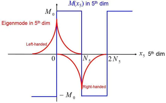
where the last two terms are the kinetic and the mass terms in the fifth dimension. In this formalism, x5-dependent mass M(x5) is introduced as shown in Fig.7, where
M0 = |M(x5)| = O(a−1) is taken to be large. Since ˆK5 includes only kinetic and
mass terms on the extra coordinate x5, the eigenvalue problem is easily solved in the
fifth direction. In this construction, there appear chiral zero modes [38, 39], i.e., a left-handed zero mode localized around x5 = 0 and a right-handed zero mode localized
aroundx5 =N5, as shown in Fig.7. The extra degrees of freedom in the fifth dimension
can be integrated out in the generating functional, with imposing the Pauli-Villars regularization to remove the UV divergence.
For the five-dimensional DW fermion kernel ˆK5, we define its eigenmode |νi and
eigenvalue Λν as
Note that each term of ˆK5 in Eq.(40) connects only the neighboring site or acts on the
same site in the five-dimensional space-time, and we can use almost the same technique as the Wilson fermion case. We consider the functional trace on a lattice withNt= 4l+1,
J ≡Tr( ˆU42l+1Kˆ52l)≃X
Figure 7. The construction of the domain wall (DW) fermion by introducing the fifth dimension ofx5and thex5-dependent massM(x5). There appear left- and
right-handed chiral zero modes localized aroundx5= 0 andx5=N5, respectively.
apart from an O(a) error, one finds [29]
LP ∝
X
ν
Λν2lhν|Uˆ42l+1|νi. (43)
After integrating out the extra degrees of freedom in the fifth dimension in the generating functional, one obtains the four-dimensional physical-fermion kernel ˆK4 [39].
The physical fermion mode is given by the eigenmode |nii of ˆK4 with its eigenvalue ˜λn, ˆ
K4|nii=i˜λn|nii, λ˜n∈C. (44)
We find that the four-dimensional physical fermion eigenvalue ˜λnof ˆK4 is approximatly
expressed with the eigenvalue Λν of the five-dimensional DW kernel ˆK5 as [29]
Λν = ˜λnν +O(M
−2
0 ) = ˜λnν +O(a
2). (45)
Combining with Eq.(43), apart from an O(a) error, we obtain [29]
LP ∝
X
ν ˜
λ2nlνhhν|Uˆ42l+1|νii, (46)
and find small contribution from low-lying physical-fermion modes of ˆK4 to the Polyakov
loop LP, due to the suppression factor ˜λ2nlν in the sum.
6. The Wilson loop and Dirac modes on arbitrary square lattices
In the following, we investigate the role of low-lying Dirac modes to the Wilson loop W, the inter-quark potential V(R) and the string tension σ (quark confining force), on
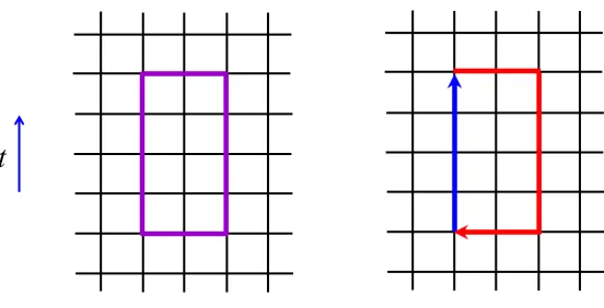
arbitrary square lattices with any number ofNt [28]. We note that the ordinary Wilson loop of theR×T rectangle on thet-xk (k = 1,2,3) plane is expressed by the functional trace,
where the “staple operator” ˆUstaple is defined by
ˆ
Ustaple ≡UˆkRUˆ−T4Uˆ−Rk. (48) In fact, the Wilson-loop operator is factorized to be a product of ˆUstaple and ˆU4T, as
shown in Fig.8.
Figure 8. (a) The Wilson loopW on aR×T rectangle. (b) The factorization of the Wilson-loop operator as a product of ˆUstaple≡UˆkRUˆ−T4Uˆ−Rk and ˆU4T [28]. Here, R, T
and the lattice sizeN3
s ×Ntare arbitrary.
6.1. Even T case
In the case of even number T, we consider the functional trace,
J ≡Trc,γ( ˆUstapleD6ˆ
where we use the completeness of the Dirac mode, P
n|nihn| = 1. With a parallel argument in Sec. 3, one finds at each lattice gauge configuration
J = 1
where, to form a loop in the functional trace, ˆU4 has to be selected in all the
ˆ
6
D ∝ P
µγµ( ˆUµ − Uˆ−µ) in ˆD6 T
. All other terms correspond to non-closed lines and give exactly zero, because of the definition of ˆU±µ in Eq.(1). We thus obtain [28]
W = (−)
factor λT cannot be cancelled by other factors, because of the finiteness of ρ(0) and Ustaple(λ) reflecting the Banks-Casher relation and the compactness ofUstaple ∈SU(Nc).
Then, the inter-quark potential V(R) is given by
where hi denotes the gauge ensemble average. The string tension σ is expressed by
Due to the reduction factor λT
n in the sum, the string tension σ or the quark confining force is unchanged by removing low-lying Dirac-mode contributions from Eq.(53).
6.2. Odd T case
In the case of odd number T, the similar results are obtained from
J ≡Trc,γ( ˆUstapleUˆ4D6ˆ
and obtains for odd T the similar formula [28]
W = (−)
Then, the inter-quark potential V(R) and the sting tension σ are expressed as
V(R) = − lim
Owing to the reduction factor λT−1
n in the sum, which cannot be cancelled by other factors, the string tension σ is unchanged by the removal of low-lying Dirac-mode contributions from Eq.(59).
7. Summary and conclusion
the clover and the domain-wall fermion kernels, respectively, and have derived similar formulae.
For all the relations obtained here, we have found that the low-lying Dirac modes contribution is negligibly small for the confinement quantities, while they are essential for chiral symmetry breaking. This indicates no direct, one-to-one correspondence between confinement and chiral symmetry breaking in QCD. In other words, there is some independence of quark confinement from chiral symmetry breaking.
This independence seems to be natural, because confinement is realized independently of quark masses and heavy quarks are also confined even without the chiral symmetry. Also, such independence generally lead to different transition temperatures and densities for deconfinement and chiral restoration, which may provide a various structure of the QCD phase diagram.
Acknowledgments
H.S. thanks A. Ohnishi for useful discussions. H.S. and T.M.D are supported in part by the Grants-in-Aid for Scientific Research (Grant No. 15K05076) and Grant-in-Aid for JSPS Fellows (Grant No. 15J02108) from Japan Society for the Promotion of Science. K.R. and C.S. are partly supported by the Polish Science Center (NCN) under Maestro Grant No. DEC-2013/10/A/ST2/0010. The lattice QCD calculations were done with SX8R and SX9 in Osaka University.
[1] Y. Nambu, inPreludes Theoretical Physicsin honor of V.F. Weisskopf (North-Holland, 1966). [2] M.Y. Han and Y. Nambu,Phys. Rev.139, B1006 (1965).
[3] D. J. Gross and F. Wilczek,Phys. Rev. Lett.30, 1343 (1973). [4] H. D. Politzer,Phys. Rev. Lett.30, 1346 (1973).
[5] R. P. Feynman, Proc. ofHigh Energy Collision of Hadrons(Stony Brook, New York, 1969). [6] J. D. Bjorken and E. A. Paschos,Phys. Rev.185, 1975 (1969).
[7] W. Greiner, S. Schramm, and E. Stein,Quantum Chromodynamics(Springer, New York, 2007). [8] Y. Nambu and G. Jona-Lasinio,Phys. Rev.122, 345 (1961);Phys. Rev.124, 246 (1961). [9] T. Banks and A. Casher,Nucl. Phys. B169, 103 (1980).
[10] K.G. Wilson,Phys. Rev.D10, 2445 (1974).
[11] J.B. Kogut and L. Susskind, Phys. Rev. D11, 395 (1975).
[12] M. Creutz,Phys. Rev. Lett.43, 553 (1979);Phys. Rev. D21, 2308 (1980).
[13] H. -J. Rothe,Lattice Gauge Theories, 4th edition, (World Scientific, 2012) and its references. [14] F. Karsch,Lect. Notes Phys.583, 209 (2002) and references therein.
[15] Y. Aoki, Z. Fodor, S.D. Katz and K.K. Szabo,Phys. Lett.B643, 46 (2006).
[16] A. Bazavov, N. Brambilla, H.-T. Ding, P. Petreczky, H.-P. Schadler, A. Vairo and J.H. Weber,
Phys. Rev. D93, 114502 (2016).
[17] H. Suganuma, S. Sasaki and H. Toki,Nucl. Phys.B435, 207 (1995). [18] O. Miyamura,Phys. Lett.B353, 91 (1995).
[19] R. M. Woloshyn,Phys. Rev. D51, 6411 (1995).
[20] V.V. Braguta, E.-M. Ilgenfritz, A.Yu. Kotov, A.V. Molochkov and A.A. Nikolaev,Phys. Rev. D94, 114510 (2016).
[22] C. Gattringer,Phys. Rev. Lett.97, 032003 (2006);
F. Bruckmann, C. Gattringer, and C. Hagen,Phys. Lett.B647, 56 (2007). [23] F. Synatschke, A. Wipf, and K. Langfeld,Phys. Rev. D77, 114018 (2008). [24] C. B. Lang and M. Schrock,Phys. Rev. D84, 087704 (2011);
L. Ya. Glozman, C. B. Lang, and M. Schrock,Phys. Rev. D86, 014507 (2012). [25] S. Gongyo, T. Iritani and H. Suganuma,Phys. Rev.D86, 034510 (2012);
T. Iritani and H. Suganuma,Prog. Theor. Exp. Phys.2014, 033B03 (2014). [26] T. M. Doi, H. Suganuma and T. Iritani,Phys. Rev. D90, 094505 (2014).
[27] T.M. Doi, K. Redlich, C. Sasaki and H. Suganuma,Phys. Rev. D92, 094004 (2015). [28] H. Suganuma, T. M. Doi and T. Iritani,Prog. Theor. Exp. Phys.2016, 013B06 (2016).
[29] H. Suganuma, T. M. Doi, K. Redlich and C. Sasaki, Acta Phys. Pol. B Proc. Suppl. B10, 741 (2017);EPJ Web of Conf.137, 04003 (2017).
[30] P. M. Lo, B. Friman, O. Kaczmarek, K. Redlich and C. Sasaki,Phys. Rev. D88, 014506 (2013). [31] P. M. Lo, B. Friman, O. Kaczmarek, K. Redlich and C. Sasaki,Phys. Rev. D88, 074502 (2013). [32] J. Bloch, F. Bruckmann and T. Wettig,JHEP1310, 140 (2013).
[33] M. G¨ockeler, H. Hehl, P.E.L. Rakow, A. Sch¨afer, W. S¨oldner and T. Wettig, Nucl. Phys. Proc. Suppl.94402 (2001).
[34] A. Bazavovet al. [HotQCD Collaboration],Phys. Rev. D90, 094503 (2014).
[35] H.B. Nielsen and M. Ninomiya, Nucl. Phys. B185, 20 (1981); erratum: Nucl. Phys. B195, 541 (1981);Nucl. Phys. B193, 173 (1981).
[36] B. Sheikholeslami and R. Wohlert,Nucl. Phys. B259, 572 (1985).
[37] Y. Nemoto, N. Nakajima, H. Matsufuru and H. Suganuma,Phys. Rev. D68, 094505 (2003). [38] D. B. Kaplan,Phys. Lett. B288, 342 (1992).
[39] Y. Shamir, Nucl. Phys. B406, 90 (1993); V. Furman and Y. Shamir, Nucl. Phys. B439, 54 (1995).
[40] H. Neuberger,Phys. Lett. B417, 141 (1998).
![Figure 4.(a) The scatter plot of the Polyakov loop in lattice QCD. The originalfigure is taken from Ref.[33].(b) The temperature dependence of the Polyakovloop susceptibilities ratio RA ≡ χA/χL and the light-quark chiral condensate ⟨ψψ ¯⟩l,normalized to its](https://thumb-ap.123doks.com/thumbv2/123dok/2962515.1356451/11.612.141.448.81.212/polyakov-originalgure-temperature-dependence-polyakovloop-susceptibilities-condensate-normalized.webp)