DETECTION OF PLANAR POINTS FOR BUILDING EXTRACTION FROM LIDAR DATA
BASED ON DIFFERENTIAL MORPHOLOGICAL AND ATTRIBUTE PROFILES
Domen Mongus, Niko Lukaˇc, Denis Obrul, and Borut ˇZalik
Faculty of Electrical Engineering and Computer Science, Laboratory for Geometric modelling and Multimedia algorithms, University of Maribor
Smetanova 17, SI-2000 Maribor
{domen.mongus, niko.lukac, denis.obrul, zalik}@uni-mb.si http://gemma.uni-mb.si/
Commission III/3
KEY WORDS:LiDAR, mathematical morphology, segmentation, DAP, DMP, building extraction
ABSTRACT:
This paper considers a new method for building-extraction from LiDAR data. This method uses multi-scale levelling schema or MSLS-segmentation based on differential morphological profiles for removing non-building points from LiDAR data during the data denoising step. A new morphological algorithm is proposed for the detection of flat regions and obtaining a set of building-candidates. This binarisation step is made by using differential attribute profiles based on the sum of the second-order morphological gradients. Any distinction between flat and rough surfaces is achieved by area-opening, as applied within each attribute-zone. Thus, the detection of the flat regions is essentially based on the average gradient contained within a region, whilst avoiding subtractive filtering rule. Finally, the shapes of the flat-regions are considered during the building-recognition step. A binary shape-compactness attribute opening is used for this purpose. The efficiency of the proposed method was demonstrated on three test LiDAR datasets containing buildings of different sizes, shapes, and structures. As shown by the experiments, the average quality of the buildings-extraction was more than
95%, with96%correctness, and98%completeness. In terms of quality, this method is comparable withTerraScanR
, but both methods significantly differ when comparing correctness and completeness of the results.
1 INTRODUCTION
Recent advances in airborne Light Detection and Ranging (Li-DAR) technology have led to the development of accurate, reli-able, and fast data-acquisition systems that go hand-in-hand with the increasing demand for generating accurate building represen-tations (Lukaˇc et al., 2013). Over the past few years, a consid-erable number of methods have been developed for this purpose that either rely on LiDAR data alone, or fuse it with aerial im-ages. Although the latter contributes to the accuracy of building-extraction by providing supplementary information beyond the scope of LiDAR systems (e.g. surface reflectance on multiple electromagnetic spectrum bands), they may not always be avail-able and several drawbacks may be related to the noise that is present within these images, such as shadows, clouds, and high-rise buildings (Meng et al., 2009). In any case, the processing of massive amounts of geometric data, with a lack of topology as obtained by LiDAR systems, is still a challenge.
Traditionally, a normalised digital surface model (nDSM) is com-puted for this purpose by subtracting the digital terrain model (DTM) from the LiDAR point-cloud (Lohmann et al., 2000). Over the past few years, several advances in building-extraction have been made that are based on mathematical morphology. Most of these methods apply morphological operations on a2.5D grid generated from a LiDAR point-cloud in order to cope with the lack of topology. One early example was based on maximum filtering (Vosselman, 2000), and dual-rank morphological filter-ing (Lohmann et al., 2000). Tarsha-Kurdi et al. (2006) used di-rectional gradient filters on interpolated DSM for detecting off-terrain segment edges. The morphological opening was therefore applied in order to remove any pronounced segments remaining on the ground, and morphological closing for filling the gaps within non-ground segments. By using the least-square method,
the authors detected non-ground planes that belonged to build-ings. Zhang et al. (2006) used progressive morphological filter-ing (Zhang et al., 2003) to find non-ground points by gradually increasing the filtering scale, and thresholding the height differ-ences. Afterwards, the authors used region growing and plane-fitting to detect buildings’ regions. Vu et al. (2009) considered LiDAR data within a multi-scale morphological space. The au-thors analysed elevation clusters’ features across the scale-space in order to detect buildings. Meng et al. (2009) proposed ground-filtering based on the elevation differences between neighbour-ing pixels, and then removneighbour-ing the majority of non-buildneighbour-ing points using morphological operators. The remaining non-building re-gions were removed by area and compactness analysis. Chen et al. (2012) extended progressive morphological filtering for de-tecting non-ground points, where the authors applied a regional growing and adaptive random sample consensus (RANSAC) al-gorithm for the detection of buildings’ segments. They consid-ered distance, standard deviation, and normal vectors’ attributes. Recently, Cheng et al. (2013) have proposed a building extrac-tion method using the reverse iterative mathematical morpholog-ical (RIMM) algorithm. This method is an extension of (Zhang et al., 2003), as it avoids relying on a constant slope by dynamically calculating those threshold values applied regarding height dif-ferences. Although this method overcomes the problem of deal-ing with builddeal-ings of different sizes, it still uses predefined struc-turing elements and is, therefore, heavily subjected to buildings’ shapes.
in Section 3. The results are given in Section 4, whilst Section 5 concludes the paper.
2 DIFFERENTIAL PROFILES
Capital letters are used in this paper to denote binary sets and the lowercase letters denote grey-scale functions. Capital and lower-case Greek letters denote the operators. Accordingly,G={pn}
is a binary set containingN foreground pointspn ∈ E, where
n∈[1, N], andE ⊂Z2, whilstg:E →Ris a regular (grey-scale) grid given by a mapping function that maps a grid-space E to height-values from R. Traditional morphological opera-tors (Shih, 2009) are defined by a structuring elementw(orwS,
wherewis square-shaped andSis its scale), whilst attribute fil-ters (Wilkinson, 2007) are defined by a generic attribute function
Λand an attribute thresholdλ. The following notations denote the fundamental morphological operators:
• Γ(G)is a binary morphological opening acting onG, • γ(g)is a grey-scale morphological opening acting ong, • Φ(G) = Γ(GC)C
is a binary closing that is by duality prop-erty (Ouzounis and Wilkinson, 2007) equal to a complement of the opened complement ofG, and
• φ(g) =−γ(−g)is a grey-scale closing, where complement is substituted by negation.
The multi-scale grid segmentation that is the focus of this pa-per is based on a morphological concept know as a granulometry (Maragos, 1989). A granulometry is an ordered set of morpho-logical filters that reduces the content of a grid by filtering it on an increasing scale. When considering traditional morphological operators, a granulometry is defined as an ordered set of struc-turing elementsw~ = {wSi|i ∈ [0, I]}, where S0 = 0 and
Si−1 < Si. As shown by Pesaresi and Benediktsson (2001),
when registering the differences between successive members of a granulometry at a point-level, a band-pass grid decomposition is achieved known as differential morphological profiles (DMPs). Denoted asδw~, DMP essentially assigns a response-vector with
Ielements to each point by δw~(g) ={γwSi
−1(g)−γwSi(g)|i∈[1, I]}. (1)
A particular member of DMP, denoted asδw~[i](g), is referred to asith
scale-zone ofg, whilstγwSI(g) is a grid multi-scale
residual. Using similar principle, Ouzounis et al. (2012) recently extended the concept of DMPs to differential attribute profiles (DAPs). Denoted asδΛ
~λ, where~λ={λi},λ0 = 0, andλi−1 <
λi, DAP withImembers is obtained by
δΛ~λ(g) ={γ
Λ
λi−1(g)−γλi(g)|i∈[1, I]}. (2)
Those members of DAP, given byδΛ
~
λ[i](g), are considered as attribute-zones ofgandγΛ
λI(g)is a grid’s attribute residual.
How-ever, this generalisation is complicated when considering all the possible attribute functions based on which filtering can be achieved. Namely, when considering e.g. shape-attributes (for example shape-compactness), where the relationship between two con-nected regionsC′ ⊆ C
from a grid-spaceE(i.e. C′, C ⊆E) does not necessarily meanΛ(C′) < Λ(C)
, the subtractive fil-tering rule needs to be considered in order to achieve a stable decomposition (Urbach et al., 2007). For simplicity, a further
condition for complementing Equation 2 is, therefore, increasing the property ofΛgiven by
C′⊆C⇒Λ(C′)≤Λ(C). (3) A straightforward example of an increasing attribute is the area of the connected regionCfrom a grid-spaceE.
Decomposition achieved by DMPs and DAPs allows for auto-mated grid segmentation by registering two characteristic proper-ties from each response vector:
• r(g)containing the maximal response obtained at each par-ticular point, and
• q(g)containing the scale at which the maximal response has been induced.
Several approaches have been proposed based on this notion (Pe-saresi and Benediktsson, 2001; Beucher, 2007; Hern´andez and Marcotegui, 2011; Ouzounis et al., 2012). In this paper, we de-fine a mappingθw~(g) :g→(r(g), q(g))at each particular point
pas
r(g)[p] = _ i∈[1,I]
δw~[i](g)[p], (4)
q(g)[p] = _ i∈[1,I]
i|r(g)[p] =δw~[i](g)[p], (5)
whereW
is the maximum. Although the given definition is based onδw~, the same definition is used to defineθ~λΛ(g)based onδ
Λ
~λ(g).
3 THE EXTRACTION OF BUILDINGS
The proposed method operates inθw~(g)andθΛ~λ(g)scale-spaces
in order to achieve building extraction from LiDAR data. The following four steps are used:
• Initialisationarranges LiDAR points into a grid,
• removal of outliersis a data denoising step, where levelling based onθw~ is used to remove those features that are too
small to be considered as buildings,
• binarisationis a grid decomposition step, where candidates for building-regions are obtained according to their sizes and surfaces based onθΛ~λ, and
• recognition of buildings, where regions’ boundary-shapes are taken into account.
3.1 Initialisation
Since connectivity between points is required when using mor-phological operators, the input LiDAR data point-cloud is ar-ranged into a regular grid. The grid-spaceE is defined by the bounding-box of the input dataset, whilst the resolution of a grid Rgis defined according to the LiDAR point-densityDLasRg = 1.0/DL, making the accuracy of the method in geometrical terms
proportional to the data density. When there is more than one point within a particular grid-cell, the lowest point is selected as the representative pointpn∈Ein order to minimise the amount
of vegetation and the number of other non-building points above the ground, whilst an interpolation is used to define the value of empty grid-cells, i.e. g[p∗
U N DEFdenote the undefined values. Inverse distance weight-ing (IDW) was selected in our case, amongst several spatial inter-polation techniques (Chaplot et al., 2006). As explained by Lloyd (2010), IDW produces a smooth oscillation-free surface without introducing any additional outliers to the data by
g[p∗
n] = P
pn∈Wp∗ng[pn]d
−r pn
P
pn∈Wp∗nd
−r pn
, (6)
wherepnis a point from the data-sampling neighbourhoodWp ∗ n
ofp∗n,dpnis the Euclidean distance betweenp∗nandpn, andr
is the power parameter that defines the smoothness of the inter-polation. As shown by Chaplot et al. (2006), accurate results are obtained by lettingr= 2, whereWp∗
ncontains no less than the
three closest points. 3.2 Removal of outliers
This denoising step is primarily focused on filtering low and high outliers (Sithole and Vosselman, 2004; Mongus and ˇZalik, 2012). Thus, sharp peaks and steep valleys need to be considered. A lev-elling schema, know asMSLS-segmentation (Pesaresi and Benedik-tsson, 2001) is applied for their detection. Consider two DMPs obtained fromg:θw~(g)containing positive response values and
θw~(−g) containing negative response values (note that this is
equivalent to replacingγwithφin Equation 1 and multiplying the obtained responses by−1). At a particular pointpn, the
fol-lowing labelling schema is used to obtain a characteristic scale q(g)ofgand corresponding responser(g):
q(g)[pn] =
q(g)[pn] | r(g)[pn]> r(−g)[pn]
q(−g)[pn] | r(g)[pn]< r(−g)[pn] 0 | r(g)[pn] =r(−g)[pn]
, (7)
r(g)[pn] = _
{r(g)[pn], r(−g)[pn]}. (8)
Accordingly, whenq(g)[pn] =q(−g)[pn], a pointpnbelongs to
a steep valley and is a suitable candidate for a low outlier, whilst q(g)[pn] =q(g)[pn]indicates a point belonging to a sharp peak,
i.e. a suitable candidate for a height outlier. Whenq(g)[pn] = 0,
a point is not considered as a noise-point and should, therefore, not be filtered. Thus, a threshold valuet[pn]at a pointpnis, in
our case, defined as
t[pn] =
2Rg if q(g)[pn] = q(−g)[pn] 4Rg if q(g)[pn] = q(g)[pn]
∞ if q(g)[pn] = 0
. (9)
Note that a higher threshold value is used when considering con-vex peaks in order to minimise the distortions of buildings’ ge-ometries caused by the filter, whilst controlling the maximal fil-tering scalewSIcontained inw~allows manipulation over the
re-moved features. Specifically, major portions of vegetation-points can be removed by recognising them as high outliers, whilst points lying within the buildings (usually recorded when targeting glass buildings) are removed as they are recognised as low outliers. In our case,w~ ={w0, w1, ...wSI}is used, whereSI = 3.0mwas
heuristically defined. A set of outliersTois then given by
To={pn|r(g)[pn]≥t[pn]}. (10)
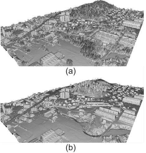
The outliers fromTo are then interpolated using eq. 6 and the
obtained result is shown in Fig. 1. 3.3 Binarisation
The binarisation step searches for flat regions ingwith areas from a predefined range, in order to obtain a set of suitable
building-(a)
(b)
Figure 1: Denoising of (a) LiDAR data generated grid, where (b) a majority of the vegetation is removed.
candidates. A new morphological algorithm is proposed that uses differential attribute profiles δΛ
~λ(g) based on attribute function Λ, defined as the sum of the second-order morphological gradi-ents. Let functions̺exand̺inestimate the external and internal
morphological gradients, respectively (Shih, 2009). The second-order morphological gradient that essentially captures the rate of change in the gradient ofg, is then estimated as̺in(̺ex(g))
. For a particular connected regionC ⊆E, a sum of gradientsΛ(C)
is obtained as
Λ(C) = X pn∈C
̺in(̺ex(g))[pn]. (11)
The points on the lower sides of the edges are emphasised, as the external gradient is computed first. Thus, flat surfaces above a neighbourhood (e.g. rooftops) have significantly lowerΛ-value than those with rough surfaces (e.g. trees). Consequently, when applying attribute openingγΛ
λbased onΛwith an attribute
thresh-oldλ, regions with larger areas are removed, if their surfaces are flat, rather than when they are rough. The ratioRa
λbetween
the areaA(C)of the removed regionsCand the value of~λ[i]
can, therefore, be used for an accurate characterisation of surface-flatness. Based on this notion, building-extraction from LiDAR data can be achieved over the following three steps:
• δΛ
~λ(g)is computed first, where the following definition of~λ
is used
~λ={0, λmin, λmin+λ∆, λmin+ 2λ∆, ..., λmax}, (12)
• each memberδΛ
~
λ[i](g)is thresholded in order to obtain a set of filtered pointsTi
Bas
TBi ={pn|δ~Λλ[i](g)[pn]>0.0}, (13)
• finally, binary area openingΓA ~ λ[i]∗Ra
λ (Ti
eachTi
Bin order to remove those regions that dissatisfy the
ratio criterionRaλ.
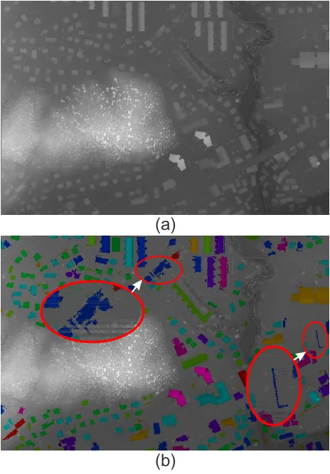
Thus, the detection of flat-regions for building-extraction is es-sentially achieved based on an average second-order morpholog-ical gradient contained within a region. Although this type of av-erage is a non-increasing attribute, the proposed framework pro-vides an elegant solution to avoid dealing with the subtractive filtering rule that is otherwise required in these cases (Urbach et al., 2007). The results obtained in the case of the test-set from Fig. 1, are shown in Fig. 2.
(a)
(b)
Figure 2: Detection of flat regions in (a) denoised gridgand (b) the results obtained based onδΛ
~λ(g), colour-coded according toi,
where~λ={0,50,100, ...,25000}was used. Two typical errors are highlighted. In the left case, points from the neighbouring vegetation are accepted as building points whilst, in the right case a brick wall with a planar top surface is accepted.
Two typical errors introduced by the proposed algorithm are high-lighted in Fig. 2b. In the first (left) case, the building-region ex-tends over the neighbouring trees, whilst a brick wall with flat top-surface was detected in the second (right) case. Both types of errors can be successfully removed during the building recog-nition step, applied over a set of building-candidatesG, obtained by
G=∪iΓ~Aλ[i]∗Ra λ(T
i
B). (14)
3.4 Recognition of buildings
In the final step of the proposed method, those flat regions that do not describe buildings are removed from the binarised grid
G. Firstly, any thin portions of regions that may extend from the buildings over the neighbouring objects (e.g. trees, as shown in Fig. 2b) are removed using binary morphological opening, i.eΓw3(G) is used in our case. Binary morphological closing Φw3(Γw3(G))is then applied in order to remove any holes that
may be present within the remaining regions. Finally, the shapes of the regions are considered and shape-compactness attribute opening is applied in order to remove long and thin regions. Let Cn∈Gbe a connected set of points fromG, andna
connected-set-index. The shape-compactnessΨ(Cn)ofCn is defined as
(Nixon and Aguado, 2012):
Ψ(Cn) =
4πA(Cn)
P(Cn)2
. (15)
whereA(Cn)andP(Cn)are the area and perimetre ofCn,
re-spectively. Shape-compactness attribute opening is then defined as
ΓΨψ(G) ={Cn∈G|Ψ(Cn)< ψ}. (16)
Thus, the set of building regionsGBis given by
GB= ΓΨψ(Φw3(Γw3(G))). (17)
4 RESULTS
The accuracy of the proposed method was examined on three test-cases within various urban features containing buildings of differ-ent sizes and shapes. The test datasetsDS1,DS2, andDS3were located at Ljubljana - ˇCrnuˇce, Medvode, and Maribor, in Slove-nia, respectively (DS1is shown in Fig. 2, whilstDS2, andDS3 can be seen in Fig. 3). The data-densities of the test-sets were as follows:12.35points/m2in the case of DS1,9.97points/m2 in the case of DS2, and6.31points/m2in the case of DS3. A different set of parameters was used for each test-case, as shown in Table 1.λmincorresponds to the area of the smallest building
contained within the dataset and is slightly larger in the case of DS1 than in the cases of DS2 and DS3. The minimal compactness of the building region defined byφdoes not significantly influ-ence the results. Consequentially,φ-values are relatively close, where slight differences in the definition do not contribute more than2%to the quality of the building-extraction, as shown in Ta-ble 2. However, the definition ofλ∆has a more significant influ-ence on the results as it defines the area by which a building can be attached to the ground and still successfully detected. The pro-posed method is relatively sensitive to this particular parameter as a largerλ∆-value increases the probability of false-positives (e.g. detection of plateaus), whilst lowerλ∆-values increases the probability of false-negatives (e.g. attached buildings).
Table 1: Parameters used for buildings-extraction from LiDAR test datasets.
Symbol Description DS1 DS2 DS3
λmin Minimal attribute value 30 20 20
λmax Maximal attribute value 40000 40000 40000
λ∆ Attribute-zone size 250 500 300 Ra
λ Attribute to area ratio 1.5 1.5 1.5
ψ Minimal compactness 9 11 10.5
The quantitative evaluation of the method was achieved by com-paring the extracted building-regions with the reference data ob-tained by the commercial softwareTerraScanR
(b) (a)
(c)
Figure 3: The results obtained by the proposed method on test-sets (a) DS1, (b) DS2, and (c) DS3, where (left) the heightmaps are coloured according to the ground-truth data. The yellow colour represents true-positives, the red colour false-positives, and the blue colour is used to show false-negatives. The extracted building points are (right) triangulated and visualised together with the generated DTM, based on Mongus and ˇZalik (2012).
considered, according to the ISPRS guidelines (Rutzinger et al., 2009):
Completeness= T P
T P+F N,
Correctness= T P
T P+F P,
Quality= Completeness−1+Correctness−1−1−1
,
whereT P,F P, andF N denote true positives, false positives, and false negatives, respectively. A comparison of the results ob-tained by the proposed method and the initial results obob-tained by TerraScanR
is shown in Table 2.
The evaluation of the proposed method showed an over 95%
average quality of building-extraction, achieving99.66% aver-age completeness and96.33%correctness. Although the aver-age quality is comparable withTerraScanR
, comparison between the completenesses and correctnesses indicates some significant differences in the performances of both methods. Namely, the proposed method achieves lower average correctness in compari-son toTerraScanR
, with the worst quality of building-extraction achieved in the case of DS1 (as shown in Figs. 1 and 2a). In comparison with DS2 and DS3, DS1 contained a considerable number of plateaus. Since some of them were recognised as buildings, the correctness of the building extraction decreased. However, this might be prevented by supplementing the method with an efficient ground-extraction algorithm (e.g. Mongus and
ˇ
Zalik (2012)). Another major contributor to errors in correctness is the fact that the proposed method does not consider a sufficient mechanism for preventing the spreading of the building-regions throughout the neighbouring objects, e.g. trees where up-to1.5m overspreading was noticed. Note that binary opening only mit-igates this problem but does not solve it. On the other hand,
TerraScanR
showed difficulties when detecting small buildings and often rejected the boundaries of larger ones. The average completeness ofTerraScanR
is, therefore, lower than the one achieved by the proposed method. However, since the proposed method is based on connected operators that are unable to break-up flzones, it is incapable of detecting buildings below the at-taching point. Consequentially, the attached buildings remained undetected (i.e. garages placed below the surrounding terrain in the case of DS2) or only partially detected (in several cases, this effect reached up to3.5m). This is the reason for the signifi-cant majority of errors in completeness introduced by the pro-posed method and can be observed in the case of DS2 (as shown in Fig.2b). On the other hand, DS3 was included within the test dataset with the purpose of examining the behaviour of the method in regard to the shapes and sizes of the contained build-ings. As shown in Fig. 3c, a great majority of errors were again related to false-positive plateaus and partially detected attached-buildings. The results, therefore, indicate that this method is ca-pable of detecting buildings of vastly different sizes and shapes. As the method achieved the worst results in the case of a test-set with the highest data-density (i.e. DS1), whilst the results are comparable in the cases of DS2 and DS3, there is no indication that the method is subjected to data density.
5 CONCLUSIONS
The paper proposes new morphological approach for the extrtion of buildings from LiDAR data. This method achieves an ac-curate removal of high and low outliers based on MSLS-segmen-tation schema, whilst a new morphological algorithm is proposed for the extraction of flat regions. Differential attribute profiles are estimated based on the sum of the second-order morphological gradients, whilst area opening performed on each attribute-zone essentially leads to the thresholding flat regions according to the average contained gradient (i.e. the ratio between the sum of gra-dients and the area of the region). Since the errors introduced by the extractions of flat regions are characteristic, they are success-fully removed according to the boundary shape during the final step of the method. Although sufficient accuracy of the proposed method was shown in comparison toTerraScanR
in all the test-cases, the great majority of errors could be related to particular limitations of the method. Namely, this method does show diffi-culties when detecting attached buildings, leading to proportional errors in the completeness of building detection, whilst errors in correctness are related to the limited detection of discontinuous terrain features (e.g. plateaus) and the overspreading of building regions throughout neighbouring vegetation. The development of sufficient solutions to these tree issues will be considered dur-ing our future work. Moreover, the mathematical stability (i.e. scale-invariance, idempotence, and increasing property) of the proposed morphological filter still needs to be proven and the ex-tension of the method for point-clouds obtained by multi-view stereo (MVS) and structure from motion (SfM) will be consid-ered.
ACKNOWLEDGEMENTS
Table 2: Quantitative evaluation of the proposed building-extraction method in comparison withTerraScanR
. TerraScanR
The proposed method Metric DS1 DS2 DS3 Average DS1 DS2 DS3 Average Completeness 96% 94% 97% 95.66% 99% 98% 99% 98.66% Corectness 97% 98% 98% 97.66% 94% 98% 97% 96.33% Quality 93% 92% 95% 93.33% 93% 96% 96% 95.00%
Development Potentials for the period2007−2013, develop-ment priority 1: Competitiveness of companies and research ex-cellence, priority axis 1.1: Encouraging competitive potential of enterprises and research excellence.
References
Beucher, S., 2007. Numerical residues. Image and Vision Com-puting 25(4), pp. 405–415.
Chaplot, V., Darboux, F., Bourennane, H., Legu´edois, S., Sil-vera, N. and Phachomphon, K., 2006. Accuracy of interpola-tion techniques for the derivainterpola-tion of digital elevainterpola-tion models in relation to landform types and data density. Geomorphology 77(1-2), pp. 126–141.
Chen, D., Zhang, L., Li, J. and Liu, R., 2012. Urban building roof segmentation from airborne lidar point clouds. International Journal of Remote Sensing 33(20), pp. 6497–6515.
Cheng, L., Zhao, W., Han, P., Zhang, W., Liu, Y. and Li, M., 2013. Building region derivation from lidar data using a re-versed iterative mathematic morphological algorithm. Optics Communications. 286, pp. 244–250.
Hern´andez, J. and Marcotegui, B., 2011. Shape ultimate attribute opening. Image and Vision Computing 29(8), pp. 533–545. Lloyd, C. D., 2010. Local Models for Spatial Analysis ( 2nd ed.).
CRC Press, Boca Raton.
Lohmann, P., Koch, A. and Schaeffer, M., 2000. Approaches to the filtering of laser scanner data. In: International Archives of Photogrammetry and Remote Sensing, Vol. 33, pp. 540–547. Lukaˇc, N., ˇZlaus, D., Seme, S., ˇZalik, B. and ˇStumberger, G.,
2013. Rating of roofs surfaces regarding their solar potential and suitability for pv systems, based on lidar data. Applied Energy 102(1), pp. 803–812.
Maragos, P., 1989. Pattern spectrum and multiscale shape repre-sentation. IEEE Transactions on Pattern Analysis and Machine Intelligence 11(7), pp. 701–715.
Meng, X., Wang, L. and Currit, N., 2009. Morphology-based building detection from airborne lidar data. Photogrammetric Engineering and Remote Sensing 75(4), pp. 437–442. Mongus, D. and ˇZalik, B., 2012. Parameter-free ground filtering
of LiDAR data for automatic DTM generation. ISPRS Journal of Photogrammetry and Remote Sensing 66(1), pp. 1–12. Nixon, M. and Aguado, A. S. (eds), 2012. Feature Extraction &
Image Processing for Computer Vision. 2nd edn, Academic Press.
Ouzounis, G. and Wilkinson, M. H., 2007. Mask-based second-generation connectivity and attribute filters. IEEE Transactions on Pattern Analysis and Machine Intelligence 29(6), pp. 990– 1004.
Ouzounis, G. K., Pesaresi, M. and Soille, P., 2012. Differential area profiles: Decomposition properties and efficient compu-tation. IEEE Transactions on Pattern Analysis and Machine Intelligence 32(8), pp. 1533–1548.
Pesaresi, M. and Benediktsson, J. A., 2001. A new approach for the morphological segmentation of high-resolution satel-lite imagery. IEEE Transactions on Geoscience and Remote Sensing 39(2), pp. 309–320.
Rutzinger, M., Rottensteiner, F. and Pfeifer, N., 2009. A com-parison of evaluation techniques for building extraction from airborne laser scanning. IEEE Journal of Selected Topics in Applied Earth Observations and Remote Sensing 2(1), pp. 11– 20.
Shih, F. Y., 2009. Image processing and mathematical morphol-ogy: fundamentals and applications. CRC Press, Boca Raton. Sithole, G. and Vosselman, G., 2004. Experimental comparison
of filter algorithms for bare earth extraction from airborne laser scanning point clouds. ISPRS Journal of Photogrammetry and Remote Sensing 59(1-2), pp. 85–101.
Tarsha-Kurdi, F., Landes, T., Grussenmeyer, P. and Smigiel, E., 2006. New approach for automatic detection of buildings in airborne laser scanner data using first echo only. In: Archives of Photogrammetry and Remote Sensing and Spatial Informa-tion Sciences, ISPRS, pp. 25–30.
Urbach, E., Roerdink, J. and Wilkinson, M., 2007. Connected shape-size pattern spectra for rotation and scale-invariant clas-sification of gray-scale images. IEEE Transactions on Pattern Analysis and Machine Intelligence 2, pp. 272–285.
Vosselman, G., 2000. Slope based filtering of laser altimetry data. In: International Archives of Photogrammetry and Re-mote Sensing, Vol. 33, pp. 935–942.
Vu, T. T., Yamazaki, F. and Matsuoka, M., 2009. Multi-scale solution for building extraction from lidar and image data. In-ternational Journal of Applied Earth Observation and Geoin-formation 11(4), pp. 281–289.
Wilkinson, M. H., 2007. Attribute-space connectivity and con-nected filters. Image and Vision Computing 25(4), pp. 426– 435.
Zhang, K., Chen, S. C., Whitman, D., Shyu, M. L., Yan, J. and Zhang, C., 2003. A progressive morphological filter for removing nonground measurements from airborne lidar data. IEEE Transactions on Geoscience and Remote Sensing 41(4), pp. 872–882.