THE USE OF LIDAR AND VOLUNTEERED GEOGRAPHIC INFORMATION TO MAP
FLOOD EXTENTS AND INUNDATION
K. McDougall a, P Temple-Watts a
a
Faculty of Engineering and Surveying, University of Southern Queensland, Toowoomba, Australia- [email protected]
KEY WORDS: Volunteered Geographic Information, LiDAR, Flood Mapping, Spatial Analysis
ABSTRACT:
Floods are one of the most destructive natural disasters that threaten communities and properties. In recent decades, flooding has claimed more lives, destroyed more houses and ruined more agricultural land than any other natural hazard. The accurate prediction of the areas of inundation from flooding is critical to saving lives and property, but relies heavily on accurate digital elevation and hydrologic models. The 2011 Brisbane floods provided a unique opportunity to capture high resolution digital aerial imagery as the floods neared their peak, allowing the capture of areas of inundation over the various city suburbs. This high quality imagery, together with accurate LiDAR data over the area and publically available volunteered geographic imagery through repositories such as Flickr, enabled the reconstruction of flood extents and the assessment of both area and depth of inundation for the assessment of damage. In this study, approximately 20 images of flood damaged properties were utilised to identify the peak of the flood. Accurate position and height values were determined through the use of RTK GPS and conventional survey methods. This information was then utilised in conjunction with river gauge information to generate a digital flood surface. The LiDAR generated DEM was then intersected with the flood surface to reconstruct the area of inundation. The model determined areas of inundation were then compared to the mapped flood extent from the high resolution digital imagery to assess the accuracy of the process. The paper concludes that accurate flood extent prediction or mapping is possible through this method, although its accuracy is dependent on the number and location of sampled points. The utilisation of LiDAR generated DEMs and DSMs can also provide an excellent mechanism to estimate depths of inundation and hence flood damage
1. INTRODUCTION 1.1 Queensland Floods
During December 2010 to February 2011, the State of Queensland experienced a series of damaging floods which caused billions of dollars in damage and the loss of over 20 lives. Major flooding was experienced at over 30 cities, towns and rural communities over southern and western Queensland including significant inundation of agricultural crops and mining communities. Consistent rain during the Australian spring resulted in many of the large catchments becoming heavily saturated and the larger storage reservoirs and dams reaching capacity.
The city of Brisbane has experienced a number of major flood events in the past. Prior to 1860, three major floods were reported for the Brisbane/Ipswich regions, with the January 1841 flood having the highest recorded level of 8.43m at Brisbane (Bureau of Meteorology, 2011b). A further five major floods inundated Brisbane and Ipswich between 1885 and 1900. In this time period, the Brisbane River peaked at 8.3m, and the Bremer River at 24.5m – its highest recorded level (Centre for the Government of Queensland, 2010). It was not until 1974 however, that Brisbane and Bremer Rivers flooded to 5.45m and 20.7m respectively – the highest levels since 1893 (Bureau of Meteorology, 2010). The 2011 Brisbane flood reached a level of 4.46m, well below the 1891 levels, but still inundating over 14,000 properties.
Early warning systems and flood models are critical in protecting the safety of citizens and property. The Queensland flood warning network derives its data from a series of rainfall and river height stations across the catchments (Bureau of Meteorology, 2011a). The Bureau of Meteorology’s Flood
Warning Centre receives the data provided by these stations and uses it in hydraulic models to produce river height predictions. In the event of an expected flood, the Flood Warning Centre issues warnings to radio stations, local government, emergency services and various other agencies involved in flood response activities. Historical data in the form of flood heights and discharge rates provide an important source of information for predicting future events.
1.2 Flood Modelling and Mapping
There has been a significant amount of research done towards the creation of flood models. Much of the work between 1999 and 2005 focused on creating models that were tested in rural areas (Ervine and Macleod, 1999; Bates and De Roo, 2000; Bates and Horritt, 2001). A number of these models were later utilised to predict flood inundation levels in urban areas (Yu and Lane, 2006; Bates and De Roo, 2000). Modelling has progressively been extended from a one dimensional (1D) to two dimensional (2D) models. A 1D model measures flood levels in the channel, whereas a 2D model measures flood depth for the extent of the floodplain.
A limit to raster-based flood models in the past has been the resolution of cells used in the model – if they are too small the computational requirements may become restrictive (Haider et al., 2003). Yu and Lane (2006) investigated the effect of model cell size for models applied to urban areas and concluded that even small variations in model resolution can have significant effects on the inundation extent. Accordingly, as processing power increases, using progressively smaller cell sizes will be a viable option. The accuracy of any flood model is dependent on the range of input data and the closeness of the model to the true behaviour of the flood water.
Mapping of the actual flood extents is often the best method of comparing these areas to determine which areas were flooded.
Three main data sources are often used to map flood extents: optical data, radar data, and topographic and river gauge data (Wang, 2002). Optical data include aerial photographs and satellite data such as from the Landsat Thematic Mapper (TM) sensor. With different reflectance responses of dry and wet/water surfaces, aerial photographs and TM data can usually distinguish between surfaces, however high turbidity can reduce the accuracy significantly. Wang (2002) also concluded that using TM data for flood extent mapping is: 1) Reliable and accurate; 2) Simply applied by using two georeferenced TM images to identify wet/dry areas, and compare before/after imagery; and 3) Efficient and cost-effective.
However, there are limitations to using many satellite sensors. As satellites have a fixed orbit pattern, their revisit time may mean data is collected long after a flood has receded. The limited spatial resolution of satellite data may also be too coarse for identifying small flooded areas, particularly in vegetated, commercial or residential areas. Additionally, the many sensors do not penetrate vegetation well, so flooding may not be reliably detected under the canopy (Wang, 2002). Finally, both optical satellite imagery and aerial photography should be collected during the day and will not penetrate cloud cover.
The same basic principle to determine flood extent i.e. detection and comparison of wet/dry surfaces before and during a flood applies also to extent mapping when using radar data. The key advantage in using synthetic aperture radar (SAR) data over optical data is the ability of radar microwave to penetrate cloud cover and forest canopies (depending on wavelength). Because current SAR sensors are satellite-mounted, these systems suffer from the same revisit time limitation as optical sensors. A number of recent satellite constellations such as COSMO-SkyMED provide targeted imagery with a revisit time of less than 12hrs (http://www.eurimage.com).
Using topographic DEMs and river gauge data is perhaps the simplest of the three methods. It requires obtaining river levels before a flood, during its peak for each gauge, and then flooding a DEM – once with the pre-flood levels, and once with peak levels. The inundated areas can then be compared to determine existing bodies of water, and flood extent (Wang, 2002). Advantages of using this approach include: 1) Data is reliable and accurate, 2) Methodology is simple, efficient, and economical, and 3) The data is easily updated. Its limitations include: only being able to map areas that have flood gauge information, and that it is sensitive to the accuracy of the input DEM.
1.3 Volunteered Information/Social Networking during the floods
As the Queensland flood events unfolded, social media and crowd sourced geographic information played an important role in keeping people informed, especially as official channels of communication began to fail or were placed under extreme load. Information and communication technologies played a critical role during the disaster and its management via the conventional communication channels such as radio, television and
newspapers but also through third party social media networks such as Twitter and Facebook.
Goodchild (2007) defines volunteered geographic information (VGI) as spatial information collected voluntarily by private citizens. Geo-tagged images submitted by individuals to the web may therefore be considered VGI. Popular examples of VGI, including: Wikimapia <http://wikimapia.org>, Flickr <http://www.flickr.com/>, and OpenStreetMap <http://www.openstreetmap.org/>. Flickr allows users to upload photos and tag them with a latitude and longitude. OpenStreetMap is ‘an editable map of the whole world, which is being built largely from scratch, and released with an open content license’ (Openstreetmap, 2011). Volunteered geographic information represents a new and rapidly growing resource which has already illustrated a myriad of uses. Its near real-time capability has been utilised in the emergency and disaster management environments to broadcast the conditions and situation on the ground (Goodchild and Glennon, 2010; De longueville et al., 2010; Zook et al., 2010; McDougall, 2011)
During the floods the Ushahidi crowd map was successfully deployed. Ushahidi is a non-profit technology company that specialises in developing free and open source software for information collection, visualisation and interactive mapping (Ushahidi, 2011). Crowdmap is an on online interactive mapping service, based on the Ushahidi platform (Crowdmap, 2011). It offered the ability to collect information from cell phones, email and the web, aggregate that information into a single platform, and visualise it on a map and timeline. Photos and videos were also able to be attached to these updates. This volunteered mapping information supplemented the informational already uploaded through Facebook, YouTube and Twitter and enabled people to connect and source updates flood level DEM. The potential of volunteered geographic information for post-disaster assessment including damage assessment, planning and official flood lines is examined.
2. METHODS 2.1 Study Site
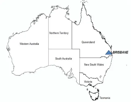
The study site consisted of an urban area in Brisbane, Australia (Figure 1) that was inundated during the recent 2011 Queensland floods. The site covered an area of 25km2 around the inner city suburbs of Brisbane and included a mixture of residential, commercial and light industrial land uses.
Figure 1. Location of study site
2.2 Data Collection
The first step of the data collection stage was to obtain private media that clearly identified the high-water mark of the January 2011 Brisbane flood. It was a requirement that these media be geo-referenced, so that their location could be readily identified. The Brisbane flood peaked at 4am on the 13th of January 2011. Some areas experienced non-riparian peaks due to local rainfall before this time. Consequently, in order to ensure the media identified the true peak flood levels, the photography needed to have been produced after 4:00am on the 13th January 2011. Where possible this was established from Exif metadata time-stamps in the image files. Where Exif tags were not present (or it was clear they were incorrect) only photos that illustrated post-peak flood marks were selected.
The vast majority of media was obtained from the online photography website flickr http://www.flickr.com. The social networking site Facebook http://www.facebook.com also provided some useful results. Finally, one image was sourced from Picasa Web http://picasaweb.google.com/. Other sources were also explored including tumblr, http://www.tumblr.com, photobucket http://photobucket.com, the image search functionality of Google http://www.google.com.au, Bing http://www.bing.com, AltaVista http://au.altavista.com, and Yahoo http://search.yahoo.com, but these sources did not provide any additional useable images not already discovered through flickr and Facebook.
In order to produce a DEM of the flood surface it was determined a minimum of 20 points across a 5km site would need to be collected. A total of 35 geo-referenced images were collected but after discounting duplicate and unsuitable images around 25 unique images remained.
Figure 2 provides an example of the imagery that was identified from the various social media soon after the flood peak. Thousands of digital photographs were taken by volunteers and published on various social media sites. Often the location of suburb and the street name have been included in the description which greatly assisted in locating these sites.
Figure 2. Volunteered image taken 14 January 2011
After the site was located from the image and supporting descriptive information, it was necessary to travel to the site to confirm the image detail. Once an image was confirmed a new digital image was recorded and the survey of the flood level was undertaken. Figure 3 illustrates a similar image taken during the GPS survey to re-create the flood peak.
Figure 4. Survey of re-located site image July 2011
A Trimble R8 GPS receiver with TSC2 controller and TDL 3G cellular modem was used in RTK mode to collect 3D coordinates for each high-water mark. The VRS or Virtual Reference System provides real-time network modelled corrections to RTK roving receivers.
The VRS corrections employed for this study were using the CMR (Compact Measurement Record) protocol, broadcast via NTRIP (Networked Transport of RTCM via Internet Protocol). The NTRIP protocol is designed to stream GNSS data over the internet. A test using two permanent marks (PM) with known coordinates confirmed the system was operating with 0.03m accuracy in the horizontal, and 0.08m in the vertical. These accuracies were considered acceptable for the study given the uncertainties in the re-construction of the flood levels.
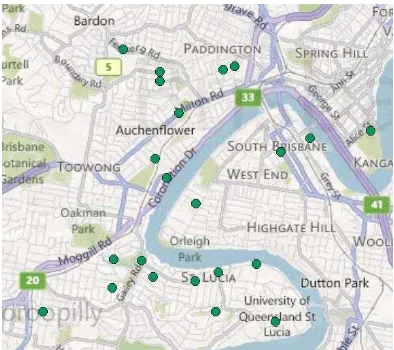
The location of the surveyed points are shown in Figure 4.
Figure 4. Distribution of the surveyed flood heights over the study area (© Microsoft Corporation 2012 and © NAVTEQ
2010)
A number of locations were unsuitable for GPS collection as the receiver was unable to gain or maintain initialisation for the selected collection time of 5 minutes. In a number of cases, reconstruction efforts meant that the high-water marks were no longer accessible, or the surface in question had been demolished. For 12 of the points, a total station was utilised to transfer a level to a location where it could not be accurately collected using GPS.
This data was then supplemented with peak water level records from Queensland Flood Warning River Height Stations for the January flood period. Australian Height Datum (AHD) data for the stations were obtained from the Bureau of Meteorology website. Water heights were then added to these AHD levels to arrive at final water levels.
LiDAR data was provided by Queensland Department of Environment and Natural Resources (DERM). The Airborne Laser Scanning (ALS) data was acquired in July 2009 using a fixed wing aircraft at a flying height of approximately 1700m with a swath width of 850m and the average point footprint of 0.34m. Laser strikes were classified into ground and non-ground points using a single algorithm across the project area. Manual checking and editing of the data classification further improved the quality of the terrain model. Thinned ground points were derived by removing superfluous points not contributing to the definition of the ground surface.
Twenty five 1km x 1km tiles of DEM and classified LAS data were utilised to cover the study area. The DEM consisted of a 1m x 1m gridded coverage for each tile with an indicative vertical accuracy of 0.15m at one sigma.
2.3 Data Processing
The ground DEM was loaded into ArcGIS and a raster DEM image was created at 5m x 5m grid interval over the study site using the kriging algorithm.. It was determined that the resolution of ground level DEM (5m x 5m) created over the study site provided an accurate representation of the terrain. A comparative analysis between the 1m and 5m grids identified that the 5m x 5m DEM compared favourably. The standard deviation between the 1m and 5m DEMs was +/- 0.07m in the flood prone areas and +/-0.37m over all terrain types. Therefore
for the purpose of flood mapping, the courser grid size was deemed appropriate.
A flood surface DEM was then generated using the 23 GPS collected flood heights. In order encompass all of the areas of inundation it was necessary to extend the flood surface DEM beyond the immediate zone of flooding. This was achieved by computing the slope of the flood surface at particular locations and using this information to establish additional DEM points where necessary. A triangulated irregular network (TIN) was established to cover the immediate flood zone and then it was clipped back to the 5km x 5km study area.
Next, using a series of raster tools in ArcGIS were utilised to compare the ground DEM with the flood surface. By subtracting the two surfaces the areas above and below the flood can be determined. The flood extents or flood lines were then computed at the change-over between the positive and negative raster values.
Finally, the areas of inundation were compared with the flood lines that were captured by the Department of Environment Natural Resources soon after the flood. The flood lines were digitised from high resolution imagery that was flown within 24hrs of the flood peak.
3. RESULTS
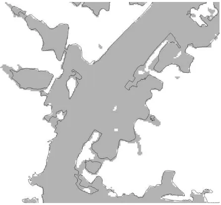
Figure 5 illustrates a hills shade interpretation of the ground surface model over the study site constructed at a 5m resolution.
Figure 5. Ground surface model of the study site using a 5m x 5m grid.
Figure 6 illustrates the flood surface created from the 23 survey points. The flood surface has a slope of approximately 2.5m over the length of the study site. The actual flood lines that were mapped shortly after the peak of the flood have been overlaid to provide context.
Figure 6. Flood surface generated from the surveyed points with the digitised flood lines overlaid.
The flood inundation area was determined by subtracting the original ground surface DEM from the flood surface model using a cut/fill algorithm. In figure 7, the outline of the digitised flood lines are overlaid to illustrate the variations between the computed and the measured. The total flooded area (including the main river) was calculated as 5.124 km2. The calculated difference between the digitised and the calculated inundation area was 0.229 km2. This represents an overall error of approximately 4.5%.
Figure 7. The derived flood inundation area with digitised flood lines overlaid
Figure 8. Depth of inundation in 1 m intervals
In addition to determining the area of inundation, the provision of accurate DEM data from LiDAR provided the ability to also determine the depth of inundation. This information is particularly useful to prioritising the risk to life and properties. For example where the depth of inundation exceeds a certain depth then it will be necessary to evacuate people from their properties. The depth of inundation is also useful for assessing the potential cost of damage to properties with higher levels of inundation increasing the cost of repairs and possible insurance claims.
4. DISCUSSION
The accurate modelling of areas that are inundated through flooding relies on the utilisation of high quality data. Two of the key sources of data for hydrological modelling are a quality DEM and an accurately modelled flood surface. The modelled flood surface is usually determined through mathematical modelling based on predicted rainfall duration and intensity, varying catchment characteristics such as land use, soil infiltration estimates, stream networks, past discharge rates, friction values and the terrain profile of the catchment. An accurate DEM is often required to both determine the slope of the terrain and also delineate the stream hierarchies. Therefore, quality DEMs are required not only for input into the hydrological model, but also to accurately interface the model results with the terrain.
The computation of the areas inundated by the 2011 flood compared closely with the flood lines that were captured soon after the flooding. With an error of less than 5% in the inundation modelling the techniques and processes are considered to be successful. This comparison does not take into consideration the error associated with the digitised flood line mapping including obstruction from buildings, vegetation and difficulty in mapping in shadow areas.
Although the inundated areas are represented with a distinct boundary there is always a degree of uncertainty (Bales et al., 2007). Uncertainty for flood inundation modelling depend a number of factors including the scale of the study (resolution), ability of the model to reflect the flood behaviour and importantly, the accuracy of the DEM.
The volunteered imagery enabled the identification of flood levels more than six months after the event and the subsequent re-construction of a flood surface. The growing utilisation of social media and sites such as Flickr, YouTube and Facebook can be successfully mined to extract useful information recorded during natural disasters.
5. CONCLUSIONS
Post flood inundation mapping is an important task in determining future flood risk, assessing insurance claims and the calibration of future hydrological models. The use of volunteered geographic information provides a growing resource for post-disaster assessment. The results from the study identified an overall error of approximately 4.5%. Therefore, in the absence of other inundation mapping data, the re-construction of inundation areas could be accurately determined through a combination of volunteered geographic information, accurate survey methods and spatial modelling techniques.
6. REFERENCES
Bales, J. D., Wagner, C. R., Tighe, K. C. and Terziotti, S., 2007.
LiDAR-derived flood-inundation maps for real-time flood mapping applications, Tar River Basin, North Carolina Scientific investigations Report 2007-5032: U.S. Geological Survey.
Bates, P. and De Roo, A., 2000. A simple raster-based model for flood inundation simulation, Journal of Hydrology., 236 (1-2), 54-77.
Bates, P. and Horritt, M., 2001. Predicting floodplain inundation: raster-based modelling versus the finite-element approach, Hydrological Processes, 15 (5), 825-842.
Bureau of Meteorology, 2010. Flood Warning System for the
Bremer River to Ipswich. Available:
http://www.bom.gov.au/hydro/flood/qld/brochures/bri sbane_bremer/bremer.shtml (15 August 2011).
Bureau of Meteorology, 2011a. Description of Queensland
Flood Warning Network Details. Available:
http://www.bom.gov.au/hydro/flood/qld/networks/des cription.shtml (10 August 2011).
Bureau of Meteorology, 2011b. Queensland Flood Summary
Pre-1860. Available:
http://www.bom.gov.au/hydro/flood/qld/fld_history/fl oodsum_pre_1860.shtml (15 August 2011).
Centre for the Government of Queensland, 2010. Queensland
Places. Available:
http://queenslandplaces.com.au/ipswich (15 August 2011).
Crowdmap, 2011. Crowdmap Website. Available: http://crowdmap.com/ (15 May 2011).
De longueville, B., Annoni, A., Schade, S., Ostlaender, N. and Whitmore, C., 2010. Digital Earth's Nervous System for crisis events: real-time Sensor Web Enablement of Volunteered Geographic Information, International Journal of Digital Earth, 3 (3), 242-259.
Ervine, A. and Macleod, A., 1999. Modelling a river channel with distant floodbanks, ICE - Water Maritime and Energy, 136 (1), 21-33.
Goodchild, M. and Glennon, A., 2010. Crowdsourcing geographic information for disaster response: a research frontier, International Journal of Digital Earth, 3 (3), 231-241.
Goodchild, M. F., 2007. Citizens as sensors: the world of volunteered geography, GeoJournal, (69), 211-221.
Haider, S., Paquier, A., Morel, R. and Champagne, J.-Y., 2003. Urban flood modelling using computational fluid dynamics, Proceedings of the ICE - Water and Maritime Engineering, 156 (2), 129-35.
McDougall, K., 2011. Understanding the Impact of Volunteered geographic Information during the Queensland Floods. Paper presented at the 7th International Symposium on Digital Earth, 23-25 August, Perth, Australia.
Openstreetmap, 2011. Openstreetmap Website (10 August 2011).
Ushahidi, 2011. Ushahidi Mission Website. Available: http://www.ushahidi.com/about-us (20 May 2011).
Wang, Y., 2002. Mapping Extent of Floods: What We Have Learned and How We Can Do Better, Natural Hazards Review, 68 (3), 68-73.
Yu, D. and Lane, S., 2006. Urban fluvial flood modelling using a two-dimensional diffusion-wave treatment, part 1: mesh resolution effects, Hydrological Processes, 20 (7), 1541-65.
Zook, M., Graham, M., Shelton, T. and Gorman, S., 2010. Volunteered Geographic Information and Crowdsourcing Disaster Relief: A Case Study of the Haitian Earthquake, Policy Studies Organisation Commons, 2 (2), 7-33.