Measurement of Elastic Strain Wave Propagation Velocity Using FRSGs along Metallic Rods Subjected to Impact Load | Sudarisman | Jurnal Semesta Teknika 727 2229 1 SM

7 7 JURNAL ILMIAH SEMESTA TEKNIKA

Vol. 13, No. 1, 77-82, Mei 2010

Measurement of Elastic Strain Wave Propagation Velocity Using FRSGs along Metallic Rods Subjected to Impact Load

(Aplikasi FRSG Untuk Pengukuran Laju Perambatan Gelombang Regangan Elastis Akibat Beban Impak pada Batang Logam)

SUDA RISMA N

ABSTRACT

The accuracy of foil resistance strain gauge (FRSG) for strain wave propagation measurement along metallic rods, i.e. aluminium, brass, copper and steel rods, subjected to impact load has been investigated. Hexagonal cross section of 5/8” sides × 6’ long metallic rods have been selected for specimens. At a distance of 8” from one end of each rod, an EA-09-125AD-120 type foil resistance strain gauge with gauge factor of 2.105 and resistance of 120Ω was installed. The rods were then placed on a pair of supports and loaded at the other end surface with an impact loading generated using an impulse hammer. The set up was also instrumented with a typical potentiometer circuit as a signal transducer, and an oscilloscope for signal acquisition. The output signals were then analysed by comparing with their respective theoretical values. The result showed that thes e FRSGs had demonstrated high accuracy in signal sensing indicated by negligible discrepancies between experimental values on one hand and their respective theor etical values on the other hand.

Keywords:FRSG, accuracy, strain wave propagation, metallic bars.

INTRODUCTION

Bonded strain gauge was firstly introduced by Charles Kearns in 1930s (Starr, 1994). It was a resistor made from combination of carbon, filler and adhesive materials. Next, in 1937 and 1938, Arthur Ruge and Edward Simons independently introduced strain gauges made of fine metal filaments (Starr, 1994). Eventually, FRSGs were introduced in the U.K. and the U.S. in the early 1950. Due to its geometry being foil with a very small cross section, a considerably small length can produce a large magnitude of resistance, and the mechanical characteristic of the specimens under investigation may not be noticeably affected. In addition, its elongation will exactly be the same as that of the specimen due to its installation being bonded. Therefore, the measurement may be guaranteed for being highly accurate.

Wide variety of strain gauges is currently available in the market. Total thickness of the

foil can be found to vary from 2.5 µm (Starr, 1994) to 10 mm with the width and length of the grids to vary from 0.51 mm to 6.35 mm and from 0.38 mm (Anonym , 2010a) to 100 mm (Anonym, 2010b), respectively. In comparison to other types of censors, FRSG

possesses some advantages, e.g., high

calibration constant stability, high accuracy, small dimension, its set up can be equipped with temperature and lead-wire compensation element, ease of installation and operation, produce linear response in wide range of measurement, can be utilised as sensing device for various transducers, and considerably low price.

Due to its superiority in comparison with other types of sensing device FGRS has widely been accepted as sensing device. Reliability of FRSG for measuring static (Sudarisman, 1998) and dynamic (Sudarisman, 2003) strains of cantilever beams has previously been reported.

strain wave propagation along metallic rods. The experimental data being captured from the pulses of elastic wave propagation signals along the rods were then compared to their respective theoretical values. The accuracy of the FRSG was calculated as the degree of discrepancy between experimental and theoretical values. The result can be used as a consideration in selecting sensing device for dynamic strain measurement.

THEORETICAL BACKGROUND

Elastic Strain Wave Propagation

The theoretical velocity of a 1-D elastic strain wave propagation along a slender metallic rod is given as (Meriam, 1980) :

vt = (E/ρ)0.5 (m/s) (1)

where E and ρ are the elastic modulus (Pa) and

density (kg/m3) of the material under

investigation. If time period of the strain wave is given as τ (s), then the frequency of the vibration is,

f = 1/τ (2)

If the length of each rod is l (m), then the wave length of the strain wave propagation is,

λ = 2l (m) (3)

Thus, the experimental value of strain wave propagation velocity in the rods is given as :

ve = 2l / τ (m/s) (4)

Foil Resistance Strain Gauge Characteristics

Charles Kearns may be the first who introduced strain gauges in 1930s (Starr, 1994). The gauges were in the form of resistors made from combination of carbon, filler and adhesive. Following him, in 1937 and 1938, Arthur C. Ruge and Edward E. Simmons , Jr. independently introduced strain gauges in the form of bonded fine metal. In 1952, Peter J. Scott Jackson invented the foil resistance gages (FRGs) that can be bonded on to the specimen being tested. These FRGs are those that currently most widely used for strain analysis and transducers.

The Measurement Group produces FRSGs whose thickness is only as thin as 2.5 – 5.0 µm, length of 0.2 – 100 mm, and resistance of 60 ? – 5000 ? (Starr, 1994). Any gauges available in the market come with specifications and detail instructio n for

installation and usage, such that by following them accurate measurement can be obtained. The shorter the applied gauge length the more

accurate a measurement, because strain

measurement using FRSGs is basically measuring strain state at a point. There are advantageous of FRSGs, e.g. stability of the constant of their circuitry, high accuracy, small in dimension, the change in temperature and the length of their lead wire can be compensated by employing compensating circuit , ease of installation and operation, linear response over a wide range of strain measurement, use ability in various types of transducer, and cost effectiveness.

Calibration is generally required for any change in circuitry variable. For signal amplifying purpose, the circuit may be equipped with a potentiometer circuit or Wheatstone bridge circuit. If a potentiometer circuit is utilised, the circuit will be equipped with a switch for connecting and disconnecting the calibration resistor.

Gauge installation is relatively easy and not time consuming. After being cleaned from mechanical and chemical contaminants, the surface where the gauge will be installed is applied with adhesive, the ga uge is carefully placed, and a light press is applied, in order to obtain a thin layer of adhesive, on to the gauge for a few minutes until the adhesive completely cured.

Potentiometer Circuit Calibration

Due to its faster response in comparison with those of Wheatstone bridge circuit, a potentiometer circuit, as presented in Figure 1, has been selecte d as the transducer in this experiment. This transducer converts elastic strain wave propagation signal into electrical voltage. In order to produce accurate measurement, the circuit has to be calibrated prior to being used for measuring elastic wave propagation signal.

The magnitude of resistance and current between points A and B are, respectively:

i = Ei / (Rb + RAB) = Ei / (RAB + Rb) (5)

When the switch S is off, i.e., loading-free state, then,

Sudarisman / Semesta Teknika, Vol. 13, No. 1, 77-82, Mei 2010 7 9

Note for Figure 1:

EA B = Eo for loading-free state

EA B = Ec for calibration loading state

EA B = Eg for actual loading state.

Ei = input voltage (V)

i = the magnitude of current in the circuit (A)

RA B = resistance between points A and B (? )

Rb = ballast resistance (? )

Rg = strain gauge resistance (? )

Rc = calibrating resistance (? )

EA B = output voltage (V)

∆Rg = the change of resistance of the strain gau ge due to loading (? )

and

EAB = Eo = iRAB = Ei / (1 + Rb/Rg) (6b)

When the switch S is on, i.e. calibration state, then :

RAB = (Rg⋅ Rc) / (Rg + Rc) (7a)

i = Ei / (Rb + RAB)

= Ei⋅(Rg⋅ Rc) /

[R

b⋅(Rg⋅ Rc) + RAB

]

(7b)

Thus,

EAB = Ec = i RAB

or

Ec = EiRc /

[

(1 + Rb/Rg) Rc + Rb

]

(8)

In measuring state where the switch S is off, then :

RAB = Rg + ∆Rg (9a)

i = Ei / (RB + RAB) = E1 /

(R

b + Rg + ∆Rg

)

(9b)

Thus,

Eg = EAB = iRAB,

or

Eg = Ei (1 + ∆Rg/Rg) /

(

1 + Rb/Rg + ∆Rg/Rg

)

(10)

If the changes of output voltage during the calibration and during loading are ∆Ec and

∆Eg, respectively, then :

∆Ec = Eo – Ec (11a)

Eg = Eo−∆Eg (11b)

If the amplitudes of the calibration and measurement signals are hc (mm) and h (mm),

respectively, then the values of calibration factor, Fc (mV/mm), and the output voltage, Eg

(mV) would be given as:

Fc = (Eo – Ec) / hc (12a)

Eg = Eo – (h/hc)(Eo – Ec) (12b)

On the substitution of equation (12b) into equation (10) produces the value of (∆Rg/Rg).

Recalling the definition of gauge factor, Fg,

(Dally et al., 1993) as:

Fg = (∆Rg/Rg) / ε (13a)

The magnitude of strain being measured, ε, can be calculated as follows:

ε = (∆Rg/Rg) / Fg (13b)

EXPERIMENT

Specimens and Instrumentation

The specimens used in the current experiment are four metallic rods made from different materials, i.e. aluminium, brass, copper and steel. The rods are of 72 (in.) long, and possessing hexagonal cross section of 11/4 (in.)

length of major diagonal. An EA-09-125AD-120 type of foil resistance strain ga uge (FRSG), supplied by the Micro-measurement Ins., was installed in each of the rods at a point of 6 (in.) from one of their respective ends. The resistance of the gauge is 120 (? ), and the gauge factor is 2.105. The main physical and mechanical properties of the specimen materials have been presented in Table 1.

FIGURE 1. Schematic diagram of a potentiometer circuit

Eo

S

Rc

Rg

Rb

Ei A

Experimental Set-up

The schematic illustration of the set-up for data acquisition has been depicted in Figure 2.

Experimental Procedure

The output voltage of the power supply was set to 6 (V), and the vertical grid lines representing time in the oscilloscope display was set to 500 (ms). Next, one of the specimens and the impulse hammer were connected to the potentiometer circuit. After the ‘TRIGGER’ button of the oscilloscope being pressed, the display would send an ‘awaiting signal’ message indicating that the oscilloscope was ready to take any input signals. The cross section of one of the specimen ends was then hit using the impulse hammer. In order to avoid bending effect, the hammer trajectory must be perpendicular to

the surface when hitting it. The strain wave propagation pattern would be displayed in output signal monitor of the oscilloscope. Immediately press the ‘STOP’ button to save the image being displayed. The image would then be traces on a peace of transparent plastic film.

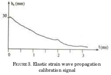
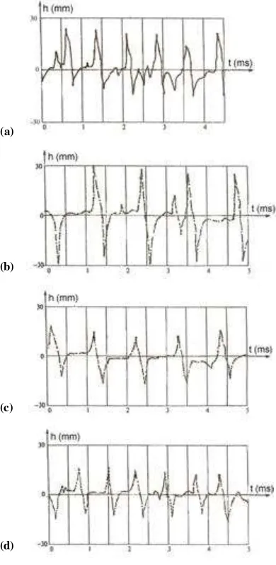
The same procedure, as above, was then applied to each of the other specimens. The calibration signal as depicted in Figure 3 can be obtained by pressing the ‘CALIBRATING SIGNAL’ button while the oscilloscope was displaying any one of the strain wave propagation signals . The elastic strain wave propagation signals of the four specimens have been presented in Figure 4.

RESULT A ND DISCUSSION

Calibration for Strain Measurement

Figure 3 below presents an elastic strain wave propagation calibration signal obtain from the experiment.

It shows that the maximum amplitude, hc, is

31 (mm). Referring to Figure 1, the values of the variables applied in this current experiment are,

Ei = 6 (V) Rg = 120 (Ω)

Rb = 120 (Ω) Rc = 120 000 (Ω)

On the substitution of these values into equations (6a), (8) and (10), yields ,

Eo = 3 (V)

Ec = 2.998 501 (V)

Eg =6 (1 + ∆Rg/Rg) /

(

2 + ∆Rg/Rg

)

(14)

Next, substitution of the values of Eo, Ec and

hc into equation (12a) gives the calibration

factor, Fc is equal to 0.046 850 (mV/mm). TABLE 1. Mechanical properties of the specimens

Material Density, ρ (g/cm3)

Young’s modulus,

E (GPa)

Poisson’s ratio,

ν Aluminium

7075-T6 2.80 70 0.33

Brass, Red

80Cu-20Zn 8.60 100 0.34

Copper,

hard 8.90 120 0.33

Steel 7.85 210 0.28

SOURCE: Gere & Timoshenko (1991)

FIGURE 2. Experimental set-up

1. Impuls hammer

2. Specimen, equipped with: (a) FRSG, (b) support system, and (c) co-axial lead -wire

3. Power supply

4. Potentiometer circuit, equipped with: (d) input voltage terminals, and (e) calibration sw itch 5. Oscilloscope, with: (f) output signal display, (g)

output signal adjustment, (h) time display adjustment, and (i) dual-channel input terminal

FIGURE 3. Elastic strain wave propagation calibration signal

1

2

a

4 3

b b

e

d

f c

g

h i

Sudarisman / Semesta Teknika, Vol. 13, No. 1, 77-82, Mei 2010 8 1

Elastic Strain Wave Propagation Speed

Figure 4 below shows strain wave propagation signals.

A vertical grid space shown in Figure 4 represents 5 (ms) time interval. It shows that the signals produced by the brass and copper bars, Figures 4(b) and 4(c), possess an almost equal time period, so do those of the aluminium and steel bars, Figures 4(a) and 4(d). Observing the signal amplitudes, hmax, the

largest one was exhibited by the elastic strain wave propagation of the brass bar, followed by that of the aluminium, and either that of the copper or steel bar.

By measuring each horizontal distance between two adjacent peak signals and

multiplying them with its time scale, i.e. 5 (ms/grid), we can obtain the time period required by each individual strain wave to propagate along each metallic rod, i.e. to travel a one complete cycle, as has been presented in column (2) of Table 2. The values of vt, as

presented in column (3) were calculated by employing equations (1) to (4), applying the constants given in Table 1, and the value for g

= 9.87 (m/s2). Next, the values of ve presented

in column (4) were obtained by multiplying the values presented in column (2) with the length of each of the metallic bars, i.e. 72 (ft).

The discrepancies presented in column (5) were considerably small, less then 4%. Experimental environment, in which the experiment were carried out might not appropriately be shielded, such as vibration of other devices, electrical and electromagnetic fields may be responsible fot this discrepancy. Such error can also come from data acquisition system, such as the length of lead-wire being used, the quality of terminal connections, as well as from the homogeneity of the materials that may affect their physical and mechanical properties.

Although the discrepancies are considerably small that indicates that strain gages demonstrated an acceptable reliability and accuracy for measuring propagation phenomena, further investigation concerning the sources of error may be worth doing. In order to enable to determine the source of such error, a study on the chemical composition and micro-structure of the material being used need to be carried out. In addition, experimental environment shielding and the sensitivity and

(a)

(b)

(c)

(d)

FIGURE 4. Elastic strain w ave propagation signals. (a) Aluminium bar, (b) Brass bar, (c) Copper bar,

and (d) Steel bar

TABLE 2. Elastic strain wave propagation speed

Material Time period,

t (ms)

Theoreti -cal speed,

v_t (m/s)

Experimen-tal speed,

v_e (m/s)

(v_e – v_t)/v_t

100%

(1) (2) (3) (4) (5)

Aluminium

7075-T 6 0.740 4990.9 4941.7 -0.986

Brass, Red

80Cu-20Zn 1.132 3336.9 3231.4 -3.161

Copper,

hard 1.043 3637.7 3505.8 -3.626

accuracy of the data acquisition system should also be a major concern.

Maximum amplitudes of the signals representing the maximum strain occurred in each bars can be obtained by measuring the

hmax of each signal as have been presented in

column (2) of Table 3. Recall that Eo = 3 (V)

and Ec = 2.998 501 (V), and substituting the

values of hmax as presented in column (2) into

equation (12b) will produced the output voltage when performing the measurement, Eg,

as presented in column (3). Next, the substitution of Eg into equation (14) yields the

values of ∆Rg/Rg as presented in column (4).

Finally, the values of maximum strain, εmax, as

presented in column (5) were obtained by employing equation (13b) for the appropriate values presented in the previous columns.

Column (5) of Table 3 reveals that an approximately the same magnitude of triggering impulses produced insignificantly different m agnitude of elastic strain among the sample bars made of different metals. These differences can only be observed after the third decimal digits of strain presented in micro-strain unit. It suggested that the differences are only in the order of 10- 10 or 10- 8 per cent, which is insignificant. Further conclusion that can be drawn is that the strain gages exhibited high accuracy for measuring elastic strain wave propagation along metallic bars.

CONCLUSION

It can be concluded that the strain gauges utilized as sensing devices for elastic strain wave measurement have demonstrated high accuracy, consistency and reliability. The

maximum discrepancies from their respective theoretical values are only 3.626% for propagation velocity measurement, and 10-8% for the magnitude measurement of elastic strain wave.

REFERENCES

Anonym. (2010a). Technical data for

general-use strain gages. Raleigh:

Micro-Measurement Inc.

Anonym. (2010b). Special use sensors –

concrete embedment strain gages.

Raleigh: Micro-Measurement Inc.

Dally, J.W., Riley, W.F. & McConnel, K.G. (1993). Instrumentation for engineering

measurements. New York: John Wiley

and Sons .

Gere, J.M. & Timoshenko, S.P. (1991).

Mechanics of materials (3rd ed.). London: Chapmann & Hall.

Meriam, J.L. (1980). Dynamics. New York:

John Wiley & Sons.

Starr, J.E. (1994). Basic strain gage

characteristics. In Hannah, R.L. and

Reed, S.E. (Ed.), Strain Gage User’s

Hanbook (pp. 1-78).London: Chapmann & Hall,.

Sudarisman. (1998). Kecermatan strain gage sebagai alat pungut sinyal regangan

statis balok kantilev er. Arena

Almamater, 12(45), 1-12.

Sudarisman. (2003). Pola regangan dinamis pada balok kantilever akibat getaran berfrekuensi renda h. Semesta Teknika, 6(1), 60-72.

AUTHOR:

Sudarisman

Department of Mechanical Engineering,

Fac ulty of Engineering, Universitas

Muhammadiyah Yogyakarta, Jalan Lingkar Selatan, Bantul 55183, Yogyakarta, Indonesia.

Email: sudarisman05@yahoo.com.au

Discussion is expected before April, 1st, 2011 and will be published in this journal on Mei 2011.

TABLE 3. Maximum elastic strain calculation