Specialty Selection and Lifetime
Returns to Specialization Within
Medicine
Jayanta Bhattacharya
A B S T R A C T
In 1995, the average American surgeon earned over $269,000 while family practice doctors earned $131,200. Using data from the Survey of Young Physicians and the American Medical Association’s Socio-Economic Monitoring Survey, I find that only half of income differences between gener-alists and specigener-alists can be explained by hours of work, residency training length, and observed and unobserved ability differences—the three competi-tive market explanations for differences in doctors’ incomes across special-ties. The most likely explanation for the remaining income differences is differential entry barriers across specialties.
A person in complete control of his mental faculties might hesitate to start to cal-culate life earnings in the different occupations. Some persons would doubt if one in partial control of his faculties would be willing for his name to appear on a document purporting to give such information. If the facts had been of less vital importance, the authors of this monograph would not have undertaken the seemingly impossible.
Harold F. Clark (1937) Jayanta Bhattacharya is an assistant professor of medicine, Center for Primary Care and Outcomes Research, Stanford University. He thanks the Agency for Health Care Policy Research, the Olin Foundation, and the Center for Economic Policy Research at Stanford University for their financial sup-port. Seminar participants at Stanford, Princeton, the University of Chicago, SUNY Stony Brook, RAND, Carnegie Mellon University, and at the 11th Annual Health Economics meetings provided helpful com-ments and suggestions. He appreciates the close reading that Partha Deb, William Sanderson, Patricia Danzon, Neeraj Sood, Darius Lakdawalla, Dana Goldman, and William Vogt gave to earlier drafts of this paper. The author thanks Marty Gaynor and an anonymous referee for useful comments and great edito-rial advice. The editoedito-rial process in this case was much more useful than is usually the case. Finally, he thanks Tom MaCurdy, Mark McClellan, and John Pencavel, who were all exceptionally helpful and patient. He claims responsibility for the remaining errors. The data used in this article can be obtained beginning in 2005 through 2008 from Jayanta Bhattacharya, Center for Primary Care and Outcomes Research, Stanford University, 117 Encina Commons, Stanford, CA 94305-6019 <jay@stanford.edu> [Submitted October 2002; accepted January 2004]
ISSN 022-166X E-ISSN 1548-8004 © 2005 by the Board of Regents of the University of Wisconsin System
I. Introduction
In 1995, the average American surgeon earned more than $269,000, while the average family practice doctor earned $131,200.1While these incomes place
even the worst paid practicing doctors in one of the best compensated professions in the United States, there are inarguably large differences in income across specialties within medicine. Such large differences seem odd in light of the fact that alldoctors undergo their most rigorous selection process in the competition to enter medical school, rather than during specialty selection.2
There are at least four possible explanations for such large premiums:
• First, surgeons and other specialist physicians tend to work longer hours than do generalist physicians—specialists would earn a higher salary even at the same wage.
• Second, specialists spend more years in residency and fellowship training than generalists; the higher salaries may be a compensating differential for these extra years.
• Third, even before any training takes place, some people may be better suited to perform the activities of a specialist than others. Being a specialist might require more dedication to keeping up with new scientific and clinical devel-opments, a sunny temperament that more happily puts up with irregular sched-ules, more manual dexterity, or even just a higher IQ. As long as these attributes are relatively rare in the population, those activities that require them will enjoy a salary premium.
• Finally, despite my curt dismissal of the possibility in the first paragraph, the residency selection process at the end of medical school may form a substan-tial barrier to entry into the specialized branches of medicine.
The purpose of this paper is to determine the extent to which differences in physician incomes are explained by the first three competitive market explana-tions. If these three explain most of the differences, there is little room for the hypothesis that specialist physician labor markets are anti-competitive, at least relative to generalist physician markets. In addition to inherent scientific interest, such a conclusion would have policy implications. For example, if specialist branches are not relatively anticompetitive, then policies encouraging the substi-tution of generalist physicians for specialists, such as paying part of the educa-tional debt of students who choose to be generalists, will yield limited medical care expenditure savings.
Economists have long been interested in doctors’ incomes. Adam Smith (1976 [1776]) emphasizes the second explanation—a compensating wage differential for greater training demands. He argues that doctors persistently earn more than “common The Journal of Human Resources
116
1. These data are from the Socioeconomic Characteristics of Medical Practice (1997).
labour,” despite free entry into the “ingenious arts and liberal professions,” because learning to be a doctor is inherently difficult; so wages must be higher to induce any-one to undergo the “tedious and expensive” training.
In their classic study of professional occupations, Friedman and Kuznets (1945) emphasize the third explanation—skill differences between specialists and general-ists. They conclude that years of experience and other observables explain about 40 percent of the income differences between specialist and generalist physicians. “Presumably, the differences that remain are largely attributable to differences in training and skill...[M]en who specialize would probably earn higher incomes as gen-eral practitioners than those who remain gengen-eral practitioners. The higher incomes of specialists are probably not a transitory phenomenon that will lead to or be eliminated by a rush to specialization; but rather a permanent concomitant of a segregation of practitioners by criteria related to their chances of success.” (Friedman and Kuznets 1945, p.278)3
As Clark (1937) notes, there are many difficulties in correctly estimating the returns to specialization. First, wage paths over the doctor’s entire career must be calculated. A static measurement would be useless as a guide to predicting the effect of policies designed to alter occupational choices. Second, an accounting must be made for unob-served abilities that determine both specialty selection and the wage path within the specialty. The crucial counterfactual question is: How much would a specialist physician make as a generalist?
The modern literature on the returns to specialization within medicine—starting with Sloan (1970)—has alternatively ignored the problems caused by either the need for lifetime wage measurement or by differential specialty selection. There is no esti-mate available of lifetime rates of return when specialty choice is jointly determined with wage. Hay (1980) estimates a joint specialty selection and wage model for physi-cians, but the partial specification of errors he uses does not permit him to calculate all opportunity costs. Hay relies on a cross-sectional data set to estimate his model, and does not explore the implications of his results for relative lifetime returns to spe-cialization. By contrast, Marder and Wilkie (1991) estimate lifetime rates of return, but they assume that specialty choice is exogenous.
This paper combines these two elements—endogenous specialty choice and life-time wages—in a single framework. A payoff for combining these elements is that this paper can answer whether surgeons and other specialists really are better at every-thing than their generalist colleagues, or just better at their particular specialties. Another related payoff is the development of some evidence on how female and minority physicians’ earnings differ from those of white and male physicians.4The
final payoff is an estimate of how important competitive market explanations are in determining the relative lifetime compensation of specialists and generalists.
3. Their more famous conclusion in this study emphasizes the fourth explanation—noncompetitive physi-cian labor markets—for the differences between doctor and lawyer compensation.
4. If there are group differences, one obvious possibility is labor market discrimination. Questions of dis-crimination are closely intertwined with questions of competition as disdis-crimination is most likely to thrive in anti-competitive environments.
II. Background
Getting into medical school requires a bachelor’s degree from a four-year college or university.5While there has been some research regarding the
effect of undergraduate education on physician specialty choice—see Ernst and Yett (1985)—such work is not conclusive, and it seems likely that most students enter medical school undecided about their specialty, or at least receptive to new experience.
Once in medical school, the first two years are devoted to the basic sciences: anatomy, physiology, biochemistry, pathology, and the rest. Clinics are usually deferred until the final two years of school and represent the student’s first prolonged contact with the various specialties of medicine.6Most schools require months in
general surgery, internal medicine, pediatrics, family practice or ambulatory medi-cine, psychiatry, and obstetrics and gynecology. Students typically explore clinical electives, including subspecialties, during the fourth year.
During the fourth year, students apply and interview for residency spots. For most students, a computerized algorithm assigns a residency position; this algorithm takes into account students’ stated preferences, as well as those of the residency programs.7
Accepting the match means agreeing to at least a three-year commitment, depending on the specialty.
Internship is the first year of residency. At the end of the internship year, a doctor completes all requirements for a license to practice medicine. Physicians with a license are legally enabled to practice general medicine, though few do.8Board
certi-fication is more rigorous and requires completing both the residency program and testing by specialty boards.
There are two routes to subspecialty training: completion of a residency program in a specialized branch of medicine, or completion of a subspecialty fellowship after fin-ishing a basic residency. Total training times, set by specialty boards, vary widely; for example, internal medicine and pediatrics take three years, radiology takes four years, and surgery takes at least five years. Fellowships in specialized fields, like cardiology or neurosurgery, can take many years after a basic residency like internal medicine or general surgery.
III. Empirical Model
A doctor’s specialty and hours of work are the outcome of choices made in a specialized labor market. Econometric work estimating the determinants of
5. There are exceptions, such as a combined six-year undergraduate and medical school program, which I will ignore as such programs are not the norm.
6. Increasingly, medical schools have been incorporating clinical instruction into the first two years. 7. There is an extensive and well-developed literature on the residency matching process. Roth (1984, 1986) has done the most prominent work on this subject (see also Roth and Peranson, 1999). Rejecting the com-puter assignment is rare because it entails a frantic search for open residency slots—there are only a few months between the match and the beginning of residency.
8. The market for licensed physicians with a single year of residency is thin.
equilibrium wage must explicitly recognize that specialty choice is, in fact, a choice, or risk incorrect inferences. In this section, I specify a joint econometric model of spe-cialty choice and wage determination in the context of utility maximizing behavior by the doctor.
In this model, I allow five aggregated specialty categories: General Practice and Family Practice (hereafter FP), Internal Medicine/Pediatrics (IM), Surgery, Inter-nal Medicine and Pediatrics Subspecialties (IM Subspecialties), and Radiology and Other Specialties (Radiology). Appendix Table 1 describes the grouping of specialties.9
First, I need some notation. Let sbe the index over the five specialties, tbe time between the date of the survey interview and medical school completion, and ibe the index over the set of all doctors. There are five potential wage streams (one for each specialty) but only the wage stream in the chosen specialty is realized. Let
{wsit}s=1f5 represent these streams, let Xi represent observed time invariant covariates predicting wage, let nsit represent the unobserved determinants of wages, and let g t( ;cs, )v be a function that reflects the dependence of wages on
experience. In Xi, I include gender, race, whether the doctor graduated from a medical school in the United States rather than abroad, and years of education of the doctor’s parents.
I use overlap polynomials—a type of spline—to flexibly specify the wage-experi-ence profiles, g t( ;cs, )v. The elements of the vector cs=(cs0,cs1,cs2,cs3)
corre-spond roughly to yearly growth rates in wages in the first, second, third, and fourth decades of practice; smoothing increases with σ, which I set in advance of estimation. Appendix 1 provides details.
Let Zsirepresent specialty choice determinants known by doctor iat the end of res-idency. Specifically, these include all the variables in Xi, debt at the end of medical school (which is my main instrument), average malpractice risk within each specialty, and years of training required to complete the specialty. Finally, let hsirepresent the unobserved determinants of specialty choice. Wage streams in each specialty are set according to:
( )1 lnwsit=Xibs+g t( ;cs, )v +nsit for s=1f5
At the end of medical school, doctors make irrevocable decisions about which specialty to enter. Each specialty branch has an associated utility level, d*
si
( )2 dsi*=Zsias+hsi for s=1f5
9. This grouping is a result of the tradeoff between preserving a clean split between the generalist special-ties and the specialist specialspecial-ties, while at the same time keeping the number of specialspecial-ties low in order to reduce the computational burden of estimation, respect sample size limitations within each specialty, and make the interpretation of results simpler. I group internal medicine and pediatrics together both because they require a similar set of cognitive skills and because they have the same required number of training years. I group obstetrics/gynecology with surgery because they both require surgical skills, and often require similar irregular schedules. I group the surgical subspecialties with surgery because of the small number of surgical specialists in my sample, as well as for computational reasons to limit the number of branches I allow. The least specialized specialties are FP and IM. The other three specialty groupings typically require more specialized training, and certainly require longer residency programs.
In Equations 1 and 2, bsand asare vectors of parameters to be estimated. Each
doctor chooses a specialty, based on Equation 2, with the maximum value of the util-ity index d*si. Let d
*
i be the chosen specialty. Then for s=1f5:
( )3 d*i=s iff dsi*$dki*6k=1f5
One of the main themes of this paper is that specialty choice and the wage set-ting processes are jointly determined in the physician labor market. The empirical model, Equations 1–3, implements this theme by allowing unobserved determi-nants of wages, nsit, and the unobserved determinants of specialty selection, hsi, to be correlated. The errors in the wage and specialty choice equations are the sum of two components; the first components in the specialty choice and wage equation errors are unique to their respective equations, while the second components are common across the equation errors. I model the second component using a step function approximation to the cumulative density function of the errors, known as a discrete factor approximation. Appendix 2 discusses the use of discrete factors in selection models.
Each discrete factor has a natural interpretation as an unobserved individual char-acteristic, such as manual dexterity or patience for irregular schedules, which deter-mines the match quality between the doctor and specialty. Each specialty may reward different combination of discrete factors differently. The model includes two discrete factors, v1andv2:10
Here, the δ’s (known as factor loads) modulate the effect of each factor on each spe-cialty. I assume hsil is distributed i.i.d. Type-I extreme value and nlsit is distributed i.i.d. N( ,0v2). I assume the factors are distributed binomially, with all three error
components mutually independent:
I restrict the mean of v1andv2to zero and a variance to one, which amounts to
plac-ing some restrictions on a1k,a2k, and pk.11There is no loss of generality due to this assumption, since the discrete factors are scaled by the δ’s.
I estimate this model using maximum likelihood. Conditional on v1andv2, the
errors are independent, so the conditional likelihood function contribution for a doc-tor in specialty sis the product of the probability of choosing the specialty and the density of the wage in that specialty:
10. Allowing two points of support on the two factors allows four different “types” of physicians. In their Monte Carlo work, Mroz and Guilkey (1999) find that allowing at least three “types” is sufficient to generate estimates that are robust to selection bias.
11. These restrictions are a pp a .
1
Removing the conditioning on v1and v2makes the specialty selection and wage
com-ponents of the likelihood function contribution of doctors from specialty sno longer separable:12 Let Asbe the set of doctors who pick specialty s. Then the likelihood function is:
1
My main data source is the 1991 Survey of Young Physicians (YPS), conducted by the Robert Wood Johnson Foundation in conjunction with the American Medical Association (AMA). The data set is representative of the 1991 population of physicians under the age of 45 years with two to nine years of practice experience. Half the sample comes from a similar survey conducted in 1987, while half is drawn randomly from the AMA physician masterfile. The survey enjoyed a nearly 70 per-cent response rate—5,884 doctors with MD degrees.13 From this initial sample of
5,884, I remove all doctors who do not report income, hours of work, or any of the other variables included in the model, leaving a final sample of 4,148 doctors.14
Yearly income consists of all pre-tax monetary returns from medical practice, including pension benefits. I construct log hourly wages using the following formula, each element of which is available for everyone in the estimation sample:15
12. I use sample weights because of the sampling scheme used to collect the data set. The weights, θi, incor-porate information not available in the other covariates Xand Z. If the sample weights were not included, maximum likelihood estimation would yield biased parameter estimates even if the likelihood function were conditioned on the correct covariates. Pfeffermann (1996) formalizes this argument. He argues that includ-ing the weights yields consistent parameter estimates if the model is specified correctly and guards against some forms of model misspecification.
13. Cantor, Baker, and Hughes (1993) provide a more complete discussion of the construction of the data set, the sampling scheme, and the calculation of the sample weights.
14. It might concern some readers that so many doctors are excluded from the initial sample. In calculations not reported here, I compared what is observed about these excluded doctors with those in the included sam-ple. The two samples are quite similar with respect to personal characteristics, though a slightly higher pro-portion of doctors in the excluded sample choose FP, IM, and Radiology and a slightly lower propro-portion choose surgery and the IM subspecialties. Physicians in the estimation sample have about $7,000 higher med-ical school debt than those in the excluded sample. A detailed table is available upon request from the author. 15. I convert all monetary variables to 1990 real dollars by applying the Consumer Price Index. Because income in the 1991 YPS is denominated in 1990 dollars, all monetary variables are in the same real units.
The Journal of Human Resources
122
Table 1
Descriptive Statistics for the Various Specialties
Internal Internal
medicine/ medicine
Family Practice Pediatrics Surgery subspecialties Radiology
Standard Standard Standard Standard Standard
Variables Mean Deviation Mean Deviation Mean Deviation Mean Deviation Mean Deviation
Personal Information
Board-certified 0.88 0.33 0.83 0.37 0.78 0.42 0.93 0.27 0.81 0.38
Age 36.2 3.01 36.3 2.93 37.3 2.90 37.5 2.70 37.2 2.80
Male 0.75 0.44 0.62 0.48 0.81 0.39 0.84 0.38 0.75 0.41
USMG 0.91 0.30 0.81 0.39 0.89 0.31 0.80 0.41 0.86 0.33
White 0.92 0.27 0.86 0.35 0.89 0.32 0.87 0.34 0.90 0.29
Black 0.035 0.19 0.038 0.19 0.035 0.19 0.022 0.15 0.020 0.13
MD awarded at age 28.6 2.33 28.7 2.18 28.3 2.04 28.3 1.86 28.8 2.04
Years of residency 2.81 0.60 3.00 0.10 4.56 0.74 4.67 0.48 3.6 0.50
training
Father’s years of 14.0 3.28 14.4 2.96 14.3 2.94 14.4 2.92 14.3 2.95
education
Mother’s years of 13.4 3.18 13.6 2.88 13.7 2.72 13.7 2.84 13.5 2.68
Bhattacharya
123
Practice and financial information
Experience in practice 5.7 2.3 5.5 2.25 5.5 2.27 5.5 2.37 5.8 2.18
(years)
Debt at graduation 31.6 30.2 25.5 26.8 26.1 31.2 20.0 26.0 24.3 24.4
from medical school (thousands of $)
Income in 1990 89.7 43.3 97.6 61.6 198 117 129 82.1 137 76.3
(thousands of $)
Hours in 1990 2670 910 2600 883 2990 871 3020 905 2420 665
Wage ($ per hour) 38.8 64.3 41.7 41.5 71.1 46.6 44.4 28.1 63.0 84.8
Log(wage) 3.49 0.50 3.56 0.54 4.09 0.63 3.62 0.61 3.95 0.54
Average yearly wage growth rates between 1985 and 1995 for the 1985 cohort of physicians
<36 years (in 1985) 4.04% 2.88% 5.28% 4.74% 3.66%
36–45 years (in 1985) 3.46% 3.15% 2.56% 4.30% 3.34%
The Journal of Human Resources 124
( )9 ln(wage)=log yearly income
(number weeks of practice hours of practice per week)( )
e o
Table 1 presents descriptive statistics for the estimation sample broken down by specialty grouping.16This table confirms some well-known facts about the medical profession. Specialists’ yearly income is significantly higher than generalists’; for example, surgeons earn an average of 221 percent more than FP doctors. Also, a higher proportion of surgeons and IM Subspecialists are male, compared to doctors in FP or IM. Surgeons and IM Subspecialists work longer hours than do doctors in other specialties.
Because the YPS is limited to young physicians and does not contain some other important information, I require some other data sources. The AMA’s (1986, 1996) Socioeconomic Characteristics of Medical Practice (SCMP) report the average yearly income of all practicing doctors by specialty, as well as the annual probability of a malpractice suit in each specialty in 1985.17Various yearly ver-sions of the American Association of Medical College’s (AAMC, 1980–90) Directory of Graduate Medical Education provide information on the training years required to obtain board certification in each specialty. Information about nominal resident wages for the years 1977–89 comes from the AAMC website (http://www.aamc.org).18 I use this information to calculate physician wages during residency.
V. Identification
In this section, I introduce and justify my identification strategy. I consider in turn the unique determinants of specialty selection and of market wage setting. In a formal sense, such an argument is unnecessary since the model is identified simply by the nonlinearity of the error distributions. However, such an identification scheme would be unappealing. Ideally, to identify the selection equations, there should be some variable that determines wages but does not determine specialty selection. Similarly, to identify the wage equations, there should be some variable that exogenously sends some candidates into one
16. The contrast category for white and black throughout the paper is “other races.” This category includes mostly Asians. Hispanics are included in the white category. USMG refers to graduates of U.S. medical schools. The contrast category consists of all graduates of foreign medical schools, whether or not they were U.S. citizens at the time of medical school.
17. Because these figures are typically reported for a more disaggregated set of specialties than is used here, I average over them, weighting by the number of doctors in each specialty, to obtain these figures at the proper level of aggregation. The main difficulty with this procedure is that the SCMP does not dis-tinguish general internal medicine doctors from specialized internal medicine doctors. Thus, the weighted average from the Internal Medicine and Pediatrics categories in the SCMP is assigned to this IM category, while the Internal Medicine category in the SCMP is assigned to my IM Subspecialties cat-egory.
specialty over the others, but has little to do with the wage setting process within the specialty.19
A variable that determines wages (observed at time t) but that does not determine specialty selection is easy to find: the survey sampling year works perfectly since it could not have been foreseen when specialty was chosen. More formally, since spe-cialty selection is made at the end of medical school before any wages streams are realized, in principle the observed determinants of selection, Zsi, cannot include
{wsit} or any other variables not known at t = 0. On the other hand, Zsi should
include projected specialty specific wage streams, { [E wsit
e
Xsi]}, where Xsi is the information that doctor ihas about each specialty supon graduation. But, the com-plete set of information observed by each doctor includes only Zsi and hsi, so{Z , }
si= si hsi
X . Including information about projected wage streams in the specialty selection equations is tantamount to including functions of Zsi. Because t—the date
at which doctors’ wages were sampled—cannot belong in Zsi, it is a theoretically
defensible instrument.
Finding an instrument that identifies the wage equation is harder; an easy tem-poral argument, such as the one in the previous paragraph, is not possible. My candidate variable is medical school debt at the time of graduation. This is strongly correlated with specialty choice, as my results demonstrate. Conversely, it is at least intuitively appealing to argue that initial assets should have little to do with the unobserved determinants of equilibrium wage later in life. Medical school debt, which for many doctors is determined by the ability of their parents to pay medical school tuition, seems like it should be unrelated, or only tangen-tially related, to the skill of the doctors years after their residency training, and thus with wage.20
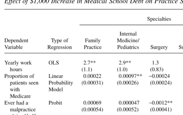
The YPS data provide some justification for this identification strategy. Table 2 shows results from regressions analyzing the effect of medical school debt on a vari-ety of medical practice style variables and an important lifestyle variable at the time of the 1991 YPS, tyears after medical school graduation. The practice style variables are yearly hours of work, proportion of patients seen with Medicare, and indicator variables for whether the doctor has ever faced a malpractice claim, whether the doc-tor is salaried, and whether the docdoc-tor is an employee of an HMO. The lifestyle vari-able is an indicator of whether the doctor in the sample is married to another doctor. Each column represents a separate set of regressions limited to physicians in the indi-cated specialty. Each cell reports the marginal effect of a $1,000 increase in medical
Bhattacharya 125
19. Heckman and Honore (1990) discuss conditions under which Roy-type selection models, such as this one, are nonparametrically identified when there is an instrument.
school debt on the row’s dependent variable. In the case of binary outcomes, for which I ran probit regressions, each cell reports marginal probability effects at the mean.21
The striking result is how little medical school debt predicts any of these practice and lifestyle outcomes. The HMO employee, salaried employee, and spouse is a doc-tor regressions have nothing but statistically insignificant and (nearly) zero estimates of the effect of debt. The debt coefficients in the yearly work hours regression for fam-ily practice doctors, internal medicine doctors, and for internal medicine specialists are statistically significant, but economically small—a $1,000 increase in debt raises hours by 2.7, 2.9, and 6.4 hours annually. The effect sizes of increasing debt by $1,000 range from 0.04 percent (for surgeons) to 0.2 percent (for internal medicine specialists) of total yearly hours. There are only two other statistically significant The Journal of Human Resources
126
21. The other variables in the regression are age, age2, male, dad’s years of education, mom’s years of
edu-cation, USMG, race dummies, and a dummy for board certification. These regression results are available upon request.
Table 2a
Effect of $1,000 Increase in Medical School Debt on Practice Style
Specialties Internal
Dependent Type of Family Medicine/ Medical
Variable Regression Practice Pediatrics Surgery Subspecialties Radiology
Yearly work OLS 2.7** 2.9** 1.3 6.4** 1.6
hours (1.1) (1.0) (0.83) (1.5) (1.1)
Proportion of Linear 0.00022 0.00097** −0.00024 0.00041 0.000040 patients seen Probability (0.00031) (0.00026) (0.00024) (0.00043) (0.00031) with Model
Medicare
Ever had a Probit 0.00069 0.000047 −0.0012** 0.00051 0.00045 malpractice (0.00054) (0.00052) (0.00041) (0.00073) (0.00051) claim filed?
HMO employee? Probit 0.000059 −0.00015 −0.00017 −0.00022 −0.00034
(0.00015) (0.00013) (0.00015) (0.00026) (0.00029) Salaried Probit 0.00046 −0.00056 0.00040 −0.00021 −0.00015
physician? (0.00061) (0.00055) (0.00047) (0.00089) (0.00059) Spouse is a Probit −0.000081 −0.00038 0.00078 0.00056 −0.00032
doctor?b (0.00062) (0.00048) (0.00043) (0.00068) (0.00056)
* 0.01<p<0.05 ** p<0.01
a. Each row in the table reports the marginal effect of a $1,000 increase in medical school debt on the row’s dependent variable. In the case of the probit regressions, each row reports marginal probability effects at the mean. Each column represents a separate regression limited to physicians in the indicated specialty. The other variables in the regression are age, age2, male, dad’s years of education, mom’s years of education,
USMG, race dummies, and a dummy for board certification. The regression coefficients for these other vari-ables are available upon request.
coefficients for debt: in the proportion of patients seen with Medicare regression for IM/Peds doctors, and in the malpractice claim regression for surgeons. Both are precisely measured zeroes.22
VI. Cohort Wage Growth Restrictions
While I am interested in lifetime specialty specific wage paths, my data set consists of a single cross-section of doctors with fewer than ten years prac-tice experience. Let observed wage growth rates in each specialty for the first, second, third, and fourth decades of doctors’ careers growth rates be ls0,ls1,ls2, and ls3
respectively (where sindexes over the five specialties). Using only the information in the YPS, only cs0—the growth rate in wages over the first decade post-residency—is
identified (by ls0). Any identification of the growth parameters after the first decade
of practice (cs1,cs2,cs3) come from the smoothing in the overlap polynomial since
there are no doctors old enough in the YPS to provide information on ls1,ls2, and s3
l . In fact (cs1,cs2,cs3) are not identified at all when σ(the smoothing parameter)
approaches zero. Clearly, a cross-sectional identification strategy alone will not work—I need other information about specialty-specific differential wage growth in the out decades.
The 1986 and 1996 SCMP report the average wage by specialty in four different age categories—younger than 36 years old, between 36 and 45 years old, between 46 and 55 years old, and between 56 and 65 years old. Thus, I observe wages for the 1985 cohort of physicians both in 1985 and in 1995 after the cohort has aged ten years. The bottom rows of Table 1 report these cohort growth rates. To see how these numbers are constructed, consider a specific example—FP doctors between 36 and 46 years old in 1985. The 1986 SCMP reports the average wage of this cohort of doctors in 1985, while the 1996 SCMP reports their average wage in 1995, after they have aged 10 years. Let wage(t,a) is the average wage in year tfor age cohort a. From these two numbers a sim-ple formula yields the average yearly wage growth rate, κ, over the decade:
(10) wage(1995,a+10)=(1+l)10wage(1985, )a
This calculation implicitly assumes that the physicians in my 1990 data set will experience the same wage growth rates as the physicians in each age category did between 1985 and 1995. For example, I assume that when the physicians in my data set are 45 years old, they will experience the same wage growth as 45-year-old physi-cians did between 1985 and 1995. This assumption is false if the wage growth of physicians is subject to an idiosyncratic shock at some point in time in the future. In defense of this assumption, however, I submit that any projection of future wages would be subject to this error. In fact, this assumption is standard in other contexts— for example, life expectancy is often calculated using this assumption—and is an improvement over cross-sectionally based projections.23
Bhattacharya 127
22. The mean probability of ever having a malpractice claim filed among surgeons is 28 percent, while the mean proportion of patients seen with Medicare by IM/Peds doctors is 21 percent.
Incorporating this cohort-based, specialty-specific wage growth information requires deriving a set of restrictions on the wage growth parameters in the model. Let ws(t,a) be the average wage of physicians in specialty sat time tfor the cohort aged ayears. Since there is only a single cross-section of physicians in my data, the age of the physicians and the time in the future are not separately identified. Doctors’ years of experience, t, can be related to their current age, years of residency training in specialty s(trains), and the age they received their MD (ageMD) by the following identity:
(11) t=a-ageMD-trains
Because of this linear relationship, the age argument in ws(t,a) can be suppressed without lost generality. The growth rate in wages from year tto t+1 is given by:
( ) ( )( ) ( )
However, the SCMP wage growth data give average growth over a decade rather than over a single year, and they average over age ranges rather than over calendar time. The average yearly wage growth rate for physicians over the decade starting from ageto age+10 is given by:
where identity (Equation 11) is substituted for t.
Equation 1 of the empirical model can be used to predict ws(t) over the course of a doctor’s career. I derive cohort wage restrictions by setting the empirical model’s predictions about the average wage growth equal to the actual wage growth observed in the SCMP data. First, I set w ts( )equal to wst from Equation 1 and then plug these wages into Equation 13. All the time invariant terms in Equation 1 cancel out of both the numerator and denominator, leaving a set of three (since there are three age cohorts that I follow in the SCMP data—I do not follow the 1985 cohort of 56 to 65 year olds) restrictions on g(t;cs), the time varying determinant of log wage in
Equation 1:24
For ease of exposition, Equation 11 is not plugged in. The final parameter estimates maximize the likelihood function (Equation 8) subject to Equation 14.25
The Journal of Human Resources 128
24. It is useful to think of the YPS micro level data as identifying the physician wage level in each specialty and its growth over the first ten years of practice. The wage growth rates over the final 30 years of practice are effectively identified by the macro data from the SCMP.
25. There are several sets of additional parameter restrictions required to identify the model. First, αsmust
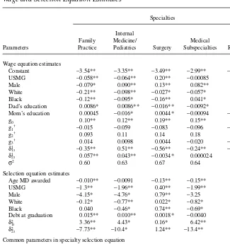
VII. Wage and Selection Equation Estimates
This section discusses the parameter estimates from the joint model of specialty choice and wage setting. The top half of Table 3 shows the wage equation results, while the bottom half shows the selection equation results.26I organize my
discussion of this table around three themes: race and gender differences in equilib-rium wage setting in medicine, other differences in wage setting, and tests of the empirical model’s validity.
A. Group Differences in Equilibrium Wage Setting
In this section, I examine racial and gender differences in wage setting within the spe-cialties of medicine. These differences are of particular interest because of the possi-bility that some groups—blacks and females in particular—face discrimination in physician labor markets. Some (like Baker, 1996) have argued that observed differ-ences across groups in the incomes of physicians are explained by differdiffer-ences in spe-cialty choices. It is clearly beyond the scope of this paper to answer whether there is discrimination against these groups in medicine, but it is entirely within its scope to document whether group-specific wage differences persist within specialties in an empirical setting aimed at accounting for unobserved skill differences. Furthermore, documenting group wage differences is closely related to the main project of this paper—a decomposition of the returns to specialization into a competitive and non-competitive part—since invidious discrimination thrives best in an anti-non-competitive environment.
I first compare the wages of black physicians with white and other race physicians. Consider the evidence from Table 3 on the generalist branches of medicine: black FP doctors earn 9 percent more than white FP doctors, while black IM doctors earn the same as white IM doctors. Other race FP doctors earn 21 percent more than white FP doctors, while other race IM doctors earn 10 percent more than white IM doctors. White, black and other race medical school graduates respond to these wage premi-ums in their specialty choices in ways one might expect—doctors of other races are 13 percent more likely than white doctors to enter FP and 116 percent more likely than white doctors to enter IM, while black doctors are more likely than whites to enter FP and IM.
Bhattacharya 129
model. Because of the presence of these conditional logit variables, one of the constants (other than in the Radiology branch) in the logit part of likelihood function must be set to zero. For the estimation, I set all the constants in the specialty selection part of the model to zero. Finally, it is not possible to estimate all the factor-loading terms, since for a given doctor, I never observe the covariance between selection probabili-ties. I arbitrarily set dk Radiology,
2
for k= 1,2 (the factor-loading terms in the Radiology specialty selection equation) equal to 0.1 to identify the model.
The pattern in the more specialized branches of medicine is not as clean. Black sur-geons earn 13 percent less than white sursur-geons, while other race sursur-geons earn 3 per-cent more than white surgeons. Nevertheless, holding all else fixed, black doctors are more likely to enter surgery than whites and doctors of other races are a little less likely to enter surgery than whites. Black IM subspecialists earn 10 percent more than white IM subspecialists, while other race IM subspecialists earn 6 percent more than white IM subspecialists. Despite this wage premium, black and white doctors are equally likely to enter the IM subspecialties. Other race doctors respond in the The Journal of Human Resources
130
Table 3
Wage and Selection Equation Estimates
Specialties Internal
Family Medicine/ Medical
Parameters Practice Pediatrics Surgery Subspecialties Radiology Wage equation estimates
Constant −3.54** −3.35** −3.49** −2.99** −3.56** USMG −0.058** −0.064** 0.20** −0.00085 0.0072
Male −0.079* 0.090** 0.13** 0.082** 0.076**
White −0.21** −0.098** −0.027* −0.057* 0.057*
Black −0.12** −0.095* −0.16** 0.041* 0.25**
Dad’s education 0.0086* 0.0086** −0.016** −0.0092* 0.011**
Mom’s education 0.00045 −0.016* 0.0044* −0.00094 −0.012*
g0 0.10** 0.12** 0.19** 0.15** 0.15*
g1† −0.015 −0.059 −0.083 −0.096 −0.092
g2† 0.093 0.11 0.14 0.18 0.15
g3† 0.014 0.0098 0.0044 −0.020 −0.0083
δ1
1s −0.35** 0.51** −0.56** −0.24** −0.60**
δ1
2s 0.057** 0.043** −0.0034* 0.000024 0.0036*
σ2 0.60 0.63 0.67 0.64 0.59
Selection equation estimates
Age MD awarded −0.010** −0.0091 −0.13** −0.15** —
USMG −1.3** −1.96** 0.40** −1.99** —
Male −4.15* −4.76* 0.79** −3.25 —
White −0.12* −0.77** 0.022* −0.82* —
Black 0.040 −0.46* 0.74** −0.69* —
Debt at graduation 0.015** 0.010** 0.0018* −0.0040 —
δ2
1s 3.36** 4.43* 0.16* 6.42** —
δ2
2s −7.73** −10.4* 1.24** −13.4** —
Common parameters in specialty selection equation
Discrete factor 1 (v1) Discrete factor 2 (v2)
Years of training 0.0023** p1 0.96** p2 0.58**
Probability of a1,1† −0.21 a1,2† −1.27
malpractice claim 1.51** a2,1† 4.90 a2,2† 0.79
* 0.01<p<0.05 ** p<0.01
expected way to their wage premium—they are 127 percent more likely than white doctors to enter the IM subspecialties. Finally, black radiologists earn 19 per-cent more than white radiologists, while other race radiologists earn 6 perper-cent less than white radiologists. Again despite this wage premium, blacks are less likely to enter radiology than whites and in accord with the wage premium, other race doctors are a little less likely than white doctors to enter radiology.
There are at least two competing explanations for the evidence on racial differences in wages across the specialties: group differences in practice style within specialties, or racial discrimination in the physician labor market. Disentangling these explana-tions is difficult without further evidence, but given the fact that black doctors on aver-age earn higher waver-ages than doctors of all other races (including whites) in IM Subspecialties and Radiology, and doctors of other races earn more than whites in four of the five specialty categories, racial discrimination seems unlikely, at least without further auxiliary and possibly ad hoc assumptions.
I turn next to gender differences: male doctors earn between 8 percent and 13 per-cent more than female doctors in all of the specialty branches, save FP, where female doctors earn 8 percent more.27Female medical graduates react to these earnings
dif-ferences by picking surgery and radiology as specialties at lower rates than men and FP at higher rates. However, women are more likely than men to pick IM and IM sub-specialties. If discrimination against female physicians is the cause of the wage dif-ferences in these specialties, such a finding (that women preferentially enter these specialties) would be odd. In IM and IM subspecialties, discrimination again seems an unlikely explanation for observed wage differences, though such a conclusion remains open in Surgery and Radiology.
B. Other Determinants of Equilibrium Wage Setting
Graduates of U.S. medical schools (USMGs) earn 6 percent less than FMGs in each of the generalist specialties, earn 20 percent more in surgery, and earn roughly the same amount in the remaining specialties. Perhaps not surprisingly, FMGs are more likely than USMGs to enter FP and IM, and 31 percent less likely to enter surgery. If there is discrimination here, it is taking place at the practice level, not at the residency selection level. Furthermore, if such discrimination handicaps FMGs in surgery, it handicaps USMGs in the generalist specialties. As before, these results do not rule out nondiscriminatory explanations.
Age at graduation has important effects on specialty selection. Compared with 35-year-old medical school graduates, doctors who enter medicine ten years earlier are 6 percent and 7 percent less likely to choose the generalist specialties FP or IM respectively, 15 percent less likely to pick Radiology, and 211 percent and 280 per-cent respectively more likely to choose Surgery or IM Subspecialties; the latter two
Bhattacharya 131
specialties require the longest training periods. Longer training periods apparently deter newly minted, but older, MDs.28
Though the malpractice coefficient reported in the specialty selection models is common across all specialty branches, the model allows changes in malpractice risk within a specialty to affect specialty selection probabilities as long as those changes are not common across specialties. However, the results imply that doubling mal-practice risk within a specialty has a near zero effect on all specialty selection proba-bilities. In some sense, this is not particularly surprising, since the existence of insurance markets against malpractice risk should blunt the effect of such risk on spe-cialty choice. This result should be of some policy interest since some have implicated increases in malpractice risk as a cause of specialist shortages.29My results indicate
that if this conclusion is true, the mechanism cannot be that malpractice risk deters young doctors from entering high risk professions.
Finally, though mothers’ and fathers’ education is sometimes statistically signifi-cant in predicting wages, the qualitative directions of these effects show no obvious pattern except that they are all small.
C. Model Validity Checks
In this section, I use the results to check two assertions that I have made. First, do the factors, v1andv2, represent components of unobserved ability, as I argue in
Section III? Second, is medical school debt strongly correlated with specialty choice, as I argue in Section V?
If the factor-loading terms in the wage equations represent the returns to unob-served abilities, then if the factor loads have the same signs and magnitudes in two different specialties, those specialties must reward the same abilities. In Table 3, the pattern of factor-loading signs shows that the first ability is rewarded posi-tively in IM and negaposi-tively in the other specialties. The second unobserved abil-ity is positively rewarded in FP and IM and has a quantitatively small effect on wages in the other specialties. This grouping provides empirical support for the notion that a different set of unobserved abilities is required to be a generalist than is required to be a specialist, and supports the interpretation of the factors as unobserved abilities.
Table 3 shows unequivocally that medical school debt is an important and statisti-cally significant predictor of specialty selection. Consider two doctors—one with $20,000 of medical school debt, one with $30,000 of debt. The doctor with the $20,000 debt is 14 percent and 9 percent less likely to FP and IM, 4 percent more likely to pick IM Subspecialties, and equally likely to pick Surgery and Radiology. The qualitative effect of debt groups together the generalist branches, and separately groups together the more specialized branches.
The Journal of Human Resources 132
28. One reason that training has a small effect is that age at graduation from medical school picks up much of the effect that the years of training variable would normally have—recall the linear relationship between age at graduation, training, and experience in Equation 10. The training variable is identified by variations in residency length within my specialty categories.
VIII. Counterfactual Lifetime Skill Premiums
Are surgeons and other specialists really more highly skilled than their generalist colleagues, or just better suited for the specialized branch of medicine they practice? The key counterfactual question is: how much would a surgeon earn as an internal medicine doctor relative to what internal medicine doctors make? In this section, I answer this question using the model of Section III to calculate the lifetime opportunity costs of picking a specialty.
A. Counterfactual wage paths
Estimating opportunity costs requires calculating alternate wage streams in each spe-cialty for each doctor starting from medical school graduation, through residency training, and up to retirement. Let Tbe the length of working life starting from med-ical school graduation.30Let these streams be denoted by ( ,t d*),
s
~ where sdenotes each of the alternate specialties, d* denotes the actually chosen specialty, and t
denotes the number of years after graduation from medical school. Thus, ~d*( ,t d*)
gives the wage path of a doctor in his chosen specialty, d*(that is, s
~ with s=d*).
Let Lsbe the length of the residency training period in each specialty. Using information from the AAMC, I set ( ,0d*)
s
~ to the real average resident wage in specialty sin the year when the doctor graduated medical school.31During
residency, wages rise by about 5 percent every year, so:
(15) ( ,t d*) ( ,0d*)( .1 05) for t 1 L and d 1 5
s = s t = f s = f
~ ~
The model predicts the alternate wage paths after residency through to retirement: *
30. I assume that each doctor retires at age 65.
1
It is difficult to compare the counterfactual wage paths across specialties because they vary across a large number of dimensions—one dimension for each year in practice. Let rbe the discount rate and H0a fixed supply of hours. The usual convention in
empirical human capital applications, which this paper follows, is to consider the net present value of income in the alternate specialties—NPV d( *)
s —as a summary index of the desirability of each occupation:32
0 0
A lifetime skill premium is defined as the percent difference between what doctors from some specialty, say d*, would earn if moved to another specialty, say s, and the
earnings of doctors who actually picked specialty s(with the earnings of doctors in specialty sas the base):
( ) ( )
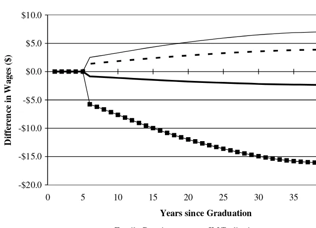
To calculate lifetime skill premiums, I first plot the difference between the projected wages of doctors from each of the alternate specialties, ( ,t d*),
s
~ and the projected wage of the doctors who chose the specialty under consideration, ~s( , )t s, at each point in time between graduation from medical school and retirement. The plots show what wages the average physician fromeach specialty would earn ineach of the alter-native specialties, from graduation to retirement. Figure 1 shows a representative plot for the five alternative wage paths of surgeons in the two-factor model. There are five such plots, one for each of the specialties.33
Table 4 shows the mean lifetime skill premiums calculated from the projected wage paths. Since the discount rate, r, is not observed, Table 4 reports the lifetime skill premium assuming r=5percent.34 These tables should be read going across rows.
Start with the lifetime skill premium of FP doctors—the first row of Table 4. Going across the row, the table reports that FPs would enjoy a statistically and economically significant 1.4 percent lifetime skill premium over IM doctors.35In other words, they
would earn morein net present value terms as IM doctors than doctors that actually chose IM earn. Continuing across the row, FP doctors would earn a positive skill pre-mium in surgery relative to practicing surgeons (2.7 percent). This should not be sur-The Journal of Human Resources
134
32. By holding hours of work fixed, NPVs(d*) ignores any labor-leisure tradeoffs. The specialty with the
largest income stream may not be the most desirable one if it requires many more hours of work than the other specialties.
33. These graphs are available from the author upon request.
34. The qualitative results are not sensitive to a range of different values of r.
35. Significance tests are reported for the H0: NPVs(d) = NPVs(s) in each cell of Table 4. Standard errors are
Bhattacharya 135
Table 4a
Lifetime Skill Premiums Relative to Doctors Who Chose the Specialty
Skill Premium Relative to Physicians in Specialty
Internal Internal Physicians in Family Medicine/ Medicine
Specialty Practice Pediatrics Surgery Subspecialties Radiology
Family practice — 1.43%† 2.74%† −9.54%** −0.42% Internal medicine/pediatrics 2.18%** — −6.30%** −11.38%** −3.84%**
Surgery 0.05% 0.07% — −3.10%** 0.08%
Internal medicine 0.63% 0.08% −0.92% — −0.96% subspecialties
Radiology 1.59%** 1.83%** 1.51% −4.78%** —
a. The table should be read going across rows. For example, in the no-selection model, family practice doc-tors would earn 0.45 percent more as internal medicine docdoc-tors than actual internal medicine docdoc-tors earn.
†0.05<p<0.1
* 0.01<p<0.05 ** p<0.01 Figure 1
Projected Difference between Wages of Doctors from Each Specialty in Surgery and Surgeon Wages
-$20.0 -$15.0 -$10.0 -$5.0 $0.0 $5.0 $10.0
0 5 10 15 20 25 30 35 40 45
Difference in Wages ($)
Family Practice IM/Pediatrics
IM Specialties Radiology and Other Specialties
prising since many Family Practice doctors (who are included in the FP category) receive some training in surgical techniques, and thus may have unobserved attributes that are similar to Surgeons.
IM doctors enjoy a 2.2 percent skill premium over FP doctors, but have large neg-ative skill premiums in all the specialized branches. There is a curiosity here: IM doc-tors would earn a positive skill premium in FP over FP docdoc-tors, and conversely FP doctors would earn a positive skill premium in IM over IM doctors. Since years of required specialty training are the same in the two specialties, from these results it may seem odd that FP doctors did not instead choose to be IM doctors, and vice versa. Such curiosities can arise in Roy-type models (such as this one) if the covariance between the unobserved determinants of returns in two specialties exceeds the vari-ance of unobserved returns in one of those specialties (see Heckman and Honoré, 1990). In that case, the average specialty-specific skills of doctors within that spe-cialty may be less than the population average level of that spespe-cialty-specific skill.
In contrast to received wisdom, surgeons earn nearly zero lifetime skill premiums in all the other specialties except in IM Subspecialties, where surgeons earn a -3 1. per-cent skill premium. Conversely, it is also not true that the lifetime skill premiums of other nonsurgical doctors in surgery are negative. The only doctors who earn statisti-cally and economistatisti-cally significant negative skill premiums in surgery are IM doctors. Though it is not true that surgeons would earn more in any other specialty than the doctors who actually picked that specialty and vice versa, there is one group of doc-tors who come close to meeting this standard. IM Subspecialists would do no worse in any alternate specialty than the average doctor in that specialty. Conversely, doc-tors from all other specialties suffer a large negative lifetime skill premium in the IM Subspecialties (that is, NPVs(IM Subspecialties) <NPVIM Subspecialties(IM Subspecialties) 6s!IM Subspecialties). Radiologists would also fare well in any spe-cialty except IM Subspecialties (relative to the doctors who chose the spespe-cialty), and no doctors would earn significantly more in radiology than radiologists.
IX. Explaining High Specialist Incomes
The motivating purpose of this paper is to estimate the importance of work hours, training-period length, and both observed and unobserved specialty selection in explaining the large differences in yearly income across medical special-ties. This section asks whether these explanations adequately describe the lifetime returns to specialization in medicine. In contrast with skill premiums, which are fea-tured in Section VIII, returns to specialization are determined by differences in coef-ficients across the specialties, rather than differences in covariates. These returns are measures of the opportunity costs for a doctor of picking a particular specialty. Consequently, this section features comparisons among the wages of a single doctor in each alternate specialty, rather than a comparison with the wages of doctors who actually chose the alternate specialty.
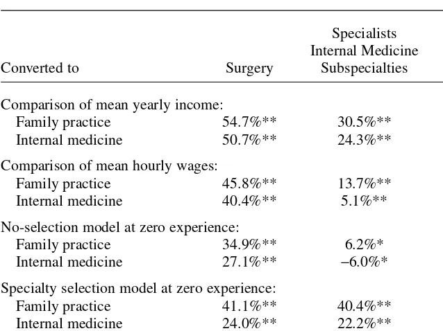
Table 5 decomposes the returns to specialization of specialists (Surgery, IM Subspecialties, and Radiology) over generalists (FP and IM). The first rows compare the unconditional mean generalist income with mean specialist income. This com-parison is often offered as support for the contention that specialists’ earnings are The Journal of Human Resources
excessive. Using this evidence, that would certainly appear to be the case. For exam-ple, FP doctors’ annual salary is 55 percent, 31 percent, and 35 percent less than Surgeons, IM Subspecialists, and Radiologists, respectively.36
The second set of rows in Table 5 compares mean hourly wages between general-ists and specialgeneral-ists, while ignoring observed and unobserved determinants of specialty selection and the evolution of lifetime earnings. Taking hours of work into account reduces the measured return to specialization in Surgery and IM Subspecialties over FP down to 46 percent and 14 percent respectively, while it raises the measured return to 38 percent in Radiology over FP. The results are similar for IM doctors. Thus, hours of work (ignoring all else) explains some of the difference in income between IM
Bhattacharya 137
36. All significance tests in Tables 5 are relative to the hypothesis of equal returns in the two specialties under consideration. All results regarding returns to specialization in this section are presented using the spe-cialized branch as a base. It may be convenient to think of the returns to specialization (for a specialist) as the losses to entering a generalist branch. Thus, with no adjustments for covariates or selection or hours of work, the mean income figures imply that Surgeons would lose 55 percent of their income if they entered Family Practice.
Table 5
Evaluating Explanations for the Returns to Specialization of Specialists over Generalists
Specialists Internal Medicine
Converted to Surgery Subspecialties Radiology
Comparison of mean yearly income:
Family practice 54.7%** 30.5%** 34.5%**
Internal medicine 50.7%** 24.3%** 28.8%**
Comparison of mean hourly wages:
Family practice 45.8%** 13.7%** 38.3%**
Internal medicine 40.4%** 5.1%** 32.2%**
No-selection model at zero experience:
Family practice 34.9%** 6.2%* 33.9%**
Internal medicine 27.1%** −6.0%* 26.0%**
Specialty selection model at zero experience:
Family practice 41.1%** 40.4%** 33.2%**
Internal medicine 24.0%** 22.2%** 13.6%**
Lifetime wage premium—two-factor model at 5% interest rate:
Family practice 31.2%** 26.8%** 16.7%**
Internal medicine 25.0%** 18.6%** 9.0%**
Subspecialists and generalists and between Surgeons and generalists, but not much of the difference between Radiologists and generalists.
The third set of rows in Table 5 shows the returns to specialization in a set of sim-ple wage regressions by specialty with no selection correction.37This row compares
the wages of generalists and specialists while adjusting for hours of work and observed covariates, but not unobserved selection or the evolution of lifetime earn-ings. Let ( ,t d*)
s
~ be the analog from these simple wage regressions to ( ,t d*),
s ~ which is the wage stream in specialty sof doctors who chose specialty d*. The third
set of rows show the predicted value of wages using these regressions of the follow-ing statistic (for s=FP, IM, and d*=Surgery, IM Subspecialties, and Radiology):38
( ) ( )
For doctors who chose specialty d*, this equation compares their projected earnings
in specialty swith their projected earnings in d*.
Controlling for observed covariates reduces the measured return to specialization for doctors in Surgery, IM Subspecialties, and Radiology over FP doctors to 35 per-cent, 6 perper-cent, and 34 percent respectively.39Similarly, for IM doctors, these controls
reduce the measured returns; in fact, for the returns of IM Subspecialists over IM doc-tors, the returns become negative—presumably there are nonpecuniary factors that induce IM Subspecialists to choose their specialty.
The fourth set of rows in Table 5 shows the added importance of unobserved spe-cialty selection over the previous set of rows, but still ignores the evolution of lifetime earnings. I calculate these numbers by replacing ~in Equation 22 with ~. The meas-ured returns of doctors in Surgery, IM Subspecialties, and Radiology over FP doctors actually increase to 41 percent, 40 percent, and 33 percent respectively relative to the no selection results. For IM doctors, however, measured returns decrease relative to surgeons and radiologists. An increase in measured returns in the selection model rel-ative to the no-selection model means that ignoring selection leads to an underesti-mateof the returns specialists earn from their unobserved specialty-specific abilities. The fifth set of rows in Table 5 shows the returns to specialization using the life-time skill premium, rather than returns to specialization at zero experience. That is, the rows present the following statistic for s=FP, IM, and d*= Surgery, IM
These final rows account for hours, length of training, and both observed and unob-served selection. Using lifetime returns rather than wages at residency graduation reduces measured returns for doctors in Surgery, IM Subspecialties, and Radiology The Journal of Human Resources
138
37. The results from these regressions, which include the same set of covariates as the wage equations reported in the paper, are available upon request from the author.
38. These rows of Table 5 report the values of No Selection Returnsd(t,s) for t= 0 (that is at zero post-residency
experience), thus ignoring how earnings change over doctors’ professional lives.
over FP doctors to 31 percent, 27 percent, and 17 percent respectively. It also reduces measured returns for surgeons and Radiologists over IM doctors, but as is the case for FP doctors, returns to specialization remain economically large.
X. Conclusion
The principal finding of this study is that hours of work, length of training, observed covariates and unobserved skill differences—the three competitive market explanations for differences in doctors’ incomes across specialties—explain only about half the differences in mean yearly income between the specialized and generalized specialties. Contrary to Friedman and Kuznets’ (1945), there remain a large part of the returns to specialization in medicine that cannot be explained by differences in training and skill.
What might explain these excess lifetime returns? First, due to data limitations, I assume that, including residency training, all doctors retire at age 65. Perhaps spe-cialties differ in the typical career lengths they support.40For example, it seems
plau-sible that surgeons retire earlier than physicians in other specialties as physical skills often deteriorate faster than mental skills with age. Unfortunately, there are no pub-lished studies comparing the career length in the various specialties, and no longitu-dinal data sets extant that would allow such a calculation. Nevertheless, because of discounting, differences in career length would most likely not change these results in any important way. At a 10 percent interest rate, an extra year of income at the end of a 40-year career is discounted by nearly 98 percent in a net present value calculation, while at a 5 percent interest rate; the extra year is discounted by nearly 86 percent.
A second possibility is that the remaining high returns of specialists are a compen-sating wage differential for unmeasured and unpleasant job characteristics or for dif-ficult to perform tasks. The selection model allows for unobserved characteristics to affect the returns in the different specialties differently, but it may not be flexible enough to account for all market relevant dimensions along which the branches of medicine differ. However, models such as the one in this paper are designed to deal with exactly this caveat. Mroz and Guilkey (1999) develop Monte Carlo evidence that discrete factor models with only a few points of support do well in accounting for unobserved characteristics in the context of a selection model such as this one. That there is some econometric reasoning available to allay concerns about this eco-nomic caveat is reassuring, but I admit that such reasoning can never be entirely con-vincing.
A third possibility is that there are barriers to entry into Surgery and Radiology that are not present in the other specialties. This explanation is plausible because the med-ical profession maintains strict control over the number available residency slots. It is the American Council on Graduate Medical Education (ACGME) that accredits resi-dency programs. The criteria for accreditation include both process planks (such as whether food service is available at the residency site, whether residents are appro-priately supervised in their activities) and substantive planks. For these latter planks,
Bhattacharya 139
ACGME requires residents in each program meet specific educational requirements (such as years of required training) that are typically set by specialty boards. Obviously, if the educational requirements set by some specialty boards are more stringent than those set by others, fewer residency programs in the selective spe-cialties will meet accreditation criteria, and all else equal there will be fewer slots available.41
If barriers to entry are the driving force behind the unexplained high returns in these specialties, then these results provide some support for the notion that specialty care is excessively priced. However, these results place strict limits on the maximum amount by which specialist wages exceed those that would obtain in a perfectly competitive market with free entry. It remains to future research to disentangle these possibilities and provide an explanation for the excess returns to specialization.
Appendix 1
Overlap Polynomial Wage Paths
I model the time varying component of wages, g(t; cs), flexibly to allow for
arbi-trary wage paths in each specialty over time. In particular, I specify gas an overlap polynomial.42The specification for g is given by:
1
where Φis the cumulative distribution function of the standard normal distribution.
sk
c should be interpreted as yearly growth rates in wages over the k+1stdecade
of a doctor’s career. The rk are analogous to the knot points in traditional splines, while the mk are analogous to the smoothing parameters. Both the rkand mk are set before estimation.43The properties of the overlap polynomial can best be appreciated
when the smoothing parameters approach zero. When this is the case, Ureduces to an indicator function equal to zero if t<rk and one if t$rk. Thus the first term of the sum, [U((t-r0)/m0)-U((t-r1)/m1)]cs0t, equals cs0t when r0<t#r1, and
zero otherwise. Thus between r0 and r1, the growth rate in log wage through time
equals cs0. Similarly, between r1and r2the growth rate is cs1, between r2 and r3it
is cs2, and between r3 and r4 it is cs3. Allowing positive values of the smoothing
parameters eliminates the sharp discontinuity of the growth rates at the knots. In fact, one advantage of this overlap polynomial over traditional splines is that the function and all its derivatives are automatically continuous at the knots without imposing any parameter restrictions.
The Journal of Human Resources 140
41. While formally voluntary, ACGME certification is important for programs because participation in the residency match and payments for medical education from Medicare are dependent upon it. In a typical year, the ACGME certifies many new programs and decertifies many existing programs. For example, in the aca-demic year 2003–04, the ACGME decertified 50 residency programs, and certified 153 new programs. 42. For a comprehensive description of overlap polynomials, see MaCurdy, Green, and Paarsch (1990), Garber and MaCurdy (1993), or Bhattacharya, Garber, and MaCurdy (1997).