Using Micro Data to Test Income Pooling
Jennifer Ward-Batts
a b s t r a c t
This paper uses an exogenous change in the intrahousehold distribution of income, provided by a change in United Kingdom Family Allowance policy to test the income-pooling hypothesis implied by unitary household models. Expenditure shares are estimated for a wide range of goods using household-level data. Shifts in expenditure shares suggest that children and mothers benefited at the expense of fathers when this policy change shifted income within households from men to women. Similar shifts are not found among married-couple households with no children. This paper refutes income pooling, and confirms and extends results in Lundberg, Pollak, and Wales (1997).
I. Introduction
In the unitary model, a household behaves like an individual, maximiz-ing a smaximiz-ingle objective function subject to a unified budget constraint. One implication of this model is that household members pool their income, so that who controls what proportion of that income does not affect household demands. Rejection of the unitary model has important implications for the effectiveness of policies aimed at improving welfare of targeted members of households. The unitary model implies neutralization of targeted transfers aimed at particular household members—a dollar of transfer
Jennifer Ward-Batts is an assistant professor of economics at Claremont McKenna College, California. She is indebted to Shelly Lundberg, Richard Startz, Robert Pollak, Terry Wales, Yoram Barzel, Elaina Rose, several anonymous referees, and numerous seminar participants for useful discussions and comments. She takes responsibility for all opinions and errors. She is grateful for support from an Alfred P. Sloan Doctoral Dissertation Fellowship while working on the earliest draft of this work, and to the Institute for Social and Economic Research at the University of Essex for their hospitality during recent work on this project. Material from the Family Expenditure Survey is Crown Copyright, has been made available by the Central Statistical Office (CSO) through the U.K. Data Archive, and has been used by permission. Neither the CSO nor the U.K. Data Archive bears any responsibility for the analysis or interpretation of the data herein. The data used in this article can be obtained by application to the U.K. Data Archive. SAS files to prepare the data can be obtained beginning October 2008 through September 2011 from Jennifer Ward-Batts, 500 E 9th St, Claremont, CA 91711, jennifer.ward-batts@cmc.edu. [Submitted August 2005; accept May 2007]
income has the same effect if transferred to the husband or to the wife. Some alternative collective models allow for more effective transfer policy.
Tests of the income-pooling hypothesis are often plagued by potential biases due to endogeneity of measures of control over income in the household. In the late 1970s, the United Kingdom changed the form of its universal child benefit scheme, essentially shifting receipt of transfer income from fathers to mothers in two-parent families. This ‘‘natural experiment’’ provides an exogenous source of variation in the control of resources within the family.
Using aggregated data, grouped by household composition and income, Lundberg, Pollak, and Wales (1997) (LPW) find that ratios of children’s to men’s and of women’s to men’s clothing expenditures in one-man, one-woman households with children in the United Kingdom increased after this policy change took effect. Hotchkiss (2005) rep-licates LPW’s results, and analyzes the aggregated data for households with no chil-dren. Similar shifts in expenditures among this group as in the treated group would cast doubt on the intrahousehold redistribution of income as an explanation for the ex-penditure shifts in families with children. Hotchkiss does find some exex-penditure shifts among households with no children, but these occurred later than those found among families with children, and well after the policy change.
In the present paper, I use household-level data to test for changes in expenditure patterns around the time of the U.K. policy change. Using household-level data, rather than the aggregated data, I am able to examine a much broader range of goods, to refine the sample of households in important ways, to better control for household demographics, time trends and seasonal variation, and to check whether a secular increase in women’s labor supply can explain the shifts in expenditures. In addition, I check, using micro data, whether similar shifts occurred in an untreated group.
Finer detail in goods and services categories is available in the micro data than in the aggregated data. Using a single-difference model in a time series of cross sections, I estimate the effect of the policy change on the share of the budget allocated to each of a comprehensive set of 11 broadly defined goods categories as well as men’s, women’s, and children’s clothing, and seven other narrowly defined goods. The hypothesis that expenditure shares for the set of broadly defined goods were unaffected by the shift in income control among families with children is strongly rejected. Controlling for pri-ces of each good, I find a decline in men’s clothing and increases in both women’s and children’s clothing—results consistent with those reported in LPW. LPW and Hotch-kiss used an aggregate clothing category price index, while this study utilizes separate price indices for each of the three clothing subcategories. Controlling for prices is im-portant since the VAT rate on children’s clothing changed relative to that on adult cloth-ing around the time of the Child Benefit policy change (Prest 1980). I also find effects among other goods that are generally in the direction we would expect. For example, I find a decrease in budget shares of alcohol and food for home preparation, and an in-crease in restaurant and take-away meals.
I also examine a sample of households with no children and do not find similar ‘‘effects’’ of this policy change for that group.1Such changes would suggest secular
shifts or some explanation for the apparent effects on families with children other than the redistribution of income within the family.
The paper is organized as follows: Section II provides some theoretical and empir-ical background motivating this research, including a discussion of the change in the Family Allowance policy. Section III discusses the data and Section IV the empirical models. Section V presents results and their implications and Section VI concludes.
II. Background
Traditional economic theory assumes each household maximizes a single objective function subject to a unified budget constraint. Samuelson (1956) suggests that this objective function might be arrived at through consensus among family members. Becker (1981) proposes it may represent the preferences of an al-truist (dictator) in the household. In these unitary models the household objective function is assumed to have the properties of a utility function and to be invariant to who controls resources in the household. One restriction implied by such models is that household members pool their resources. This pooled income is then used to maximize the household objective function. This implies that only total household income, not its distribution, affects household demands.
This has important practical implications for policies targeted at improving the wel-fare of particular household members, such as women or children. Income pooling results in transfers to targeted household members being neutralized by the house-hold-allocation mechanism. The welfare of the targeted member may be improved, but no more or less than if the transfer had been given to another household member. Cash transfers, as well as transfers in kind, may be subject to this reallocation.
Alternative theoretical models allow for the possibility that each adult in the household has distinct preferences, and provide a framework for analyzing how their competing interests are reconciled. These more general models do not impose in-come pooling. They include general collective models (for example, Chiappori 1988, 1992), and both cooperative and noncooperative bargaining models due to Manser and Brown (1980), McElroy and Horney (1981), Bergstrom (1996), and Lundberg and Pollak (1993, 1994), among others. These models allow income accru-ing to different family members to affect household demands differently. For in-stance, in cooperative Nash-bargained solutions, each person’s (potential) income affects his or her reservation level of utility either outside the marriage (divorce threat) or in a noncooperative solution inside marriage (separate spheres), and there-fore his or her equilibrium level of utility in the household. Thus, these models allow for more effective targeted transfer policies.
not subject to these concerns tend to be sporadic and insignificant. Many previous tests of pooling, including Thomas (1990), Schultz (1990), Phipps and Burton (1998), and Bourguinon et al. (1993) have used some of these potentially endogenous sources of income. These tests have generally rejected pooling, but possible endogeneity biases call those results into question. Some more recent tests have been based on policy changes generating quasi-experimental variation in the intrahousehold distribution of income.2Using data from a randomized treatment at the beginning of the Progresa program in Mexico, Attanasio and Lechene (2002) reject the income-pooling hypoth-esis. They find that increasing the wife’s share of household income increases the bud-get share allocated to children’s clothing and food and decreases the share allocated to alcohol. By contrast, Bradbury (2004) does not find evidence against income pooling in Australia when a change in unemployment benefit policy shifted most of the benefit from husbands to wives.3Bradbury suggests this may be due in part to benefits gener-ally being deposited directly into joint accounts in Australia, so that practical control of the income may not have changed. Both studies focus on a low-income sample due to the nature of the policies examined.
Moehling (2003) extends application of a collective model to include children as decision makers. She finds that, though they generally turned over earned income to parents, working children in the United States in 1917–19 gained power in household decision making by working for wages. However, Bingley and Walker (1997) find that in-kind transfers targeted at children of particular ages in the United Kingdom in more recent times were at least partly undone by the household-allocation process. These transfers may not have significantly increased outside options for recipient children, and thus may not affect a cooperatively bargained solution.
Previous empirical literature examining child outcomes and relative control over resources has generally found evidence that children do better when the mother con-trols a greater share of household resources. Thomas (1990) finds that the mother’s unearned income has a much larger positive effect on measures of child health and survival than the father’s unearned income in a sample of urban Brazilian house-holds. Thomas, Contreras, and Frankenberg (2002) find that in Java and Sumatra, mothers’ resources brought to marriage decrease episodes of illness in their sons rel-ative to daughters. They are unable to reject the unitary model in other parts of Indo-nesia. Quisumbing and Maluccio (2003) reject the unitary model in data from four countries using relative resources brought to marriage as a measure of bargaining power. In Bangladesh and South Africa, increases in female-owned assets increase expenditures on education, while it is higher men’s assets that positively affect edu-cation in Ethiopia. After public pensions were extended to blacks in South Africa, Duflo (2003) finds that pensions received by women have a large positive impact on the health of girls, but little effect on boys, while men’s pensions do not appear to impact child health.
2. An alternate strategy is to use resources brought to marriage as a measure of bargaining power exoge-nous to household decisions. For example, see Thomas, Contreras, and Frankenberg (2002) and Quisumbing and Maluccio (2003).
In the United Kingdom in the late 1970s, the child benefit scheme was altered in such a way as to shift income from fathers to mothers in two-parent households. Prior to 1977, the program consisted of a small taxable Family Allowance payment to the mother, and a more significant Child Tax Allowance, which reduced the amount of taxes withheld from earned income. The latter generally would have increased the father’s take home pay. This two-part program was phased out over the period April 1977 to April 1979 and replaced by the universal Child Benefit, a nontaxable cash payment to the mother.4 While the average amount of the total benefit remained roughly constant, this policy change shifted apparent control of a portion of family income from fathers to mothers. The amount of income involved is a significant frac-tion of the average family’s budget. For example, for a family with two children in April 1980, the Child Benefit was approximately 445 British pounds per year5 (ap-proximately 180 pounds in 1974 currency), or about 8 percent of male manual earn-ings in the United Kingdom.6The real value of that benefit is 7.5 percent of average total expenditure among families with one to three children in the data used for this study. In April 1974, the annual amount of Family Allowance paid to the mother in a two-child family was 47 pounds. Since Family Allowance was taxable and Child Benefit was not, the difference of 134 pounds in 1974 currency can be viewed as a lower bound of the amount of income shifted to the wife.
Based on this policy shift, which is clearly exogenous with respect to household expenditure decisions, LPW present empirical evidence against the pooling hypoth-esis, using grouped data on household expenditures.7 Using expenditure data from before and after the policy change, they ‘‘find strong evidence that a shift toward rel-atively greater expenditures on women’s goods and children’s goods coincided with this income redistribution.’’ (p.1) Limitations of the aggregated data dictated some shortcomings, such as a concentration on clothing, and limited demographic con-trols.8 Each cell in the data used by LPW and subsequently by Hotchkiss consists of the mean of expenditures on a category of goods for all families in the sample that fall into a particular income—family-size group. One-man, one-woman households with zero, one, two, or three children form groups from which income subgroups are created. The man and woman in these households may or may not be (living as) hus-band and wife. They may consist, for example, of an adult child and that individual’s opposite-sex parent. In addition, the small number of cells in the data makes it dif-ficult to distinguish effects of the policy change from time trends.
A potential confounder is the 1979 change in the value-added tax (VAT) rate. This rate rose from eight percent to 15 percent, and at the same time, clothing and foot-wear for young children became zero-rated. This change, occurring around the time of the change in the Child Benefit, likely affected the relative prices of adult and children’s clothing. LPW and Hotchkiss use a price index for the aggregate category, clothing and footwear. Thus, the increase they find in the ratio of children’s clothing
4. Kooreman (2000) analyzes household expenditures in the Netherlands and finds a ‘‘labeling’’ effect— that the marginal propensity to consume children’s goods out of Child Benefit income is higher than that from other types of income. However, Edmonds (2002) does not find a labeling effect in Slovenia. 5. Department of Health and Social Security (1991), Table G1.01, p. 253.
6. House of Commons (January 14, 1980, pp. 641–42).
expenditures to men’s clothing expenditures may be attributable in part to changes in relative prices for which they are unable to control. I use separate price indices for the three clothing categories in estimates presented here.
Using household-level data from the Family Expenditure Survey, I estimate budget shares for some narrow goods categories that may be of greater interest to certain members of the household, including men’s, women’s, and children’s clothing and footwear. Since the policy change gives wives control over a greater proportion of household income, we would expect to see a shift in consumption toward goods that are of relatively greater interest to wives. Such shifts would warrant a rejection of pooling, and thus provide evidence against the unitary model. The nature of these shifts also has important implications for the effectiveness of policies intended to im-prove welfare for targeted household members.
III. Data and Sample Construction
The Family Expenditure Survey (FES) is conducted annually in the United Kingdom. Ten thousand households are randomly selected each year, approx-imately 70 percent of which complete the survey. Face-to-face interviews and a two-week expenditure diary completed by each ‘‘spender’’9are used to collect detailed information on household expenditures, income, and household demographics. Some expenditure items, such as food and clothing, are covered only in the diaries. For other items, such as fuel and housing expenditures, interviews supplement informa-tion from the diaries. Expenditures are reported as weekly values.
The survey is spread over the entire the year, making it possible to control for sea-sonal effects on expenditures. The data include the region in which the household is located: Northern Ireland, Scotland, Wales, or one of nine regions in England. The data include detailed income information by source and by household member. I con-struct a set of nine dummy variables to control for household composition, catego-rizing households by the number of children in the household and their ages.
For the primary analysis, the sample is limited to households with man, one-woman who is recorded as the wife of the household head, and one to three chil-dren.10 I include only households in which the husband is younger than 65 and the wife is younger than 60 years of age in order to avoid pensioners.11This results in a total sample size of 15,753 households over eight years of data. I use data from 1973 to 1983 but drop the intermediate years, 1977–79, during which the Child Ben-efit policy change was phased in. I create three binary variables for the post-policy-change period, one for each family size, allowing for the policy to affect families of different sizes in a general way.
I also create a sample of households with a man and woman living as husband and wife in which there are no children. Like the primary sample, I exclude households in which the man is aged 65 or more, or the woman is aged 60 or more. Including
pensioners may be problematic for several reasons. A post-retirement decline in con-sumption has been documented in many developed countries, including in the United Kingdom by Banks, Blundell and Tanner (1997). Many economists have been trying to explain this consumption drop in a way that is consistent with rational forward-look-ing behavior. One possible explanation put forth for the drop is that bargainforward-look-ing power shifts in favor of the wife around retirement, due in part to the receipt of public pensions, which may increase her share of current household income. In addition, the wage of the husband relative to the wife may fall when he retires from a career job (see Lundberg 1999). Lundberg, Startz, and Stillman (2003) find evidence in support of marital bar-gaining as an explanation for the post-retirement fall in consumption.
Further, there was a drop over the period being studied here in the wife’s share of the U.K. standard married couple’s state pension.12These complexities make pen-sioners problematic for inclusion in either the treatment or the control group. After excluding pensioner households, the ‘‘untreated’’ sample contains 7,887 households over the same eight years included in the treatment group sample.
These samples differ from those used by LPW (1997) and Hotchkiss (2005). By using the published aggregated data, one is unable to distinguish ages of individual household members or their relationship to one another. The aggregated data sample will thus include many pensioners, as well as households not consisting of a married couple (or couple living as if they are married), such as siblings, or a single mother and her adult coresiding son, for example. Without the age and relationship restric-tions, the micro data sample of man-woman households with no children would be considerably larger.13
Price indices from the Abstract of National Statistics(CSO 1984–87) are used. These are available quarterly for 11 broadly defined goods categories, as well as for all goods combined (the Retail Price Index). In estimates of narrowly defined clothing expenditures, I use detailed price indices obtained from the Office for Na-tional Statistics in the United Kingdom. These indices are available monthly for a number of narrowly defined goods, including men’s clothing, women’s clothing, and children’s clothing.14The two sets of price indices come ultimately from the same source, but the latter is aggregated to a lesser degree. Neither set is available separately by region. Both are inclusive of VAT.
IV. Empirical Models
The basic empirical model is a Quadratic Almost Ideal Demand System (QAIDS). The budget share for each good can be estimated equation-by-equation using:
12. The U.K. standard pension benefit provides a fixed amount for a single individual or a married person whose spouse receives her own benefit. If only one spouse qualifies based on previous National Insurance contributions, the couple receives a married couple benefit, which was 62 percent larger than the single per-son benefit in 1970. The relative couple benefit fell 1970–76, and then leveled off at 60 percent above the single person benefit in 1977 through 1983.
wig¼ag+gglogpg+b1glog
wherewigis the budget share for good categorygfor householdi;pgis the relative price for good categoryg, computed by dividing the national price index for that cat-egory by the Retail Price Index (RPI). While inclusion of all prices is preferred, mul-ticolinearity results if all prices are included due to the short time series and absence of cross-sectional (regional) price variation. Ciis total household consumption or ex-penditure. Iiis the household-specific price index for all goods, approximated by15
logIi¼+ g
wiglogpg: ð2Þ
Addition of the square of log total consumption to the AIDS model of Deaton and Muellbauer (1980a,b), makes it more flexible, and is demonstrated to improve model fit in FES data by Banks, Blundell, and Lewbel (1997).16F andQare vectors of parameters. D is a set of three dummy variables representing the policy change for one-, two-, and three- child families.17His a vector of household demographic and other control variables, including eight of nine household composition categories grouped by number and ages of children, 11 of 12 region dummies, the quarter of the year in which the household was surveyed, and a quadratic time trend based on cal-endar year.uigis an error term with standard properties. This model can be estimated equation-by-equation using ordinary least squares regression, or by two-stage least squares (TSLS), as discussed below.
Given expenditure diary data for a two-week period, many households will record zero expenditures on some goods. The correct empirical model to apply depends on the mechanism generating those zeroes. If infrequency of purchase generates the zeroes, then the tobit model is not the correct specification. Purchase infrequency generates measurement error in the dependent variable. We want to make inference about consumption, which is rarely directly measured; instead, we measure expendi-ture. We can write the relationship of observed expenditure to unobserved consump-tion aswig¼wig+eig, whereeigis measurement error,w
*
is the latent consumption share, andwour proxy for it, the observed expenditure share. Assuming the measure-ment error is not correlated with any of the righthand side variables, then OLS can be used to estimate the model.18 However, there is reason for concern that total
15. According to Deaton and Muellbauer (1980b) this approximation was used by J. R. N. Stone. No par-ticular work is cited. I use broad category expenditure shares and corresponding price indices to calculate this index for each household.
16. This form is also used by Attanasio and Lechene (2002). I experiment with higher order polynomials in total expenditure and find the quadratic form to be the best fit.
17. Due to their low frequency in the data, larger families are omitted from the sample.
expenditure will be endogenous with respect to expenditure shares, particularly for goods of a durable or nonperishable nature, generating correlation between total ex-penditure and the measurement error in the dependent variable. Total exex-penditure will be higher in periods when a durable or nonperishable good, say, clothing, is pur-chased than in periods when it is not. A common solution to this problem in demand estimation is to use a measure of the household’s normal income to instrument for total expenditure. Keen (1986) uses ‘‘normal income’’ (based on usual rather than current earnings) to instrument for total expenditure in estimating Engel curves using a single year of FES data, and shows that this produces consistent estimates.
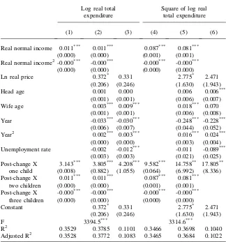
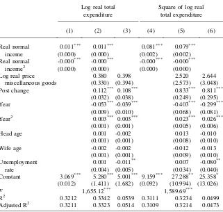
I use the same normal income measure and its square to instrument for log of total expenditure and its square in TSLS estimates.19An example of a first-stage regres-sion is shown in Appendix 1, Table A1 for families with children and in Appendix 1, Table A2 for households without children. The price in each first stage will differ depending on the good being estimated. The adjustedR-squared for the model shown is 0.377 and 0.368 for log expenditure and its square in the with-children sample, while the instruments alone explain 35.3 percent and 34.7 percent of the variation in the two endogenous variables. The corresponding adjustedR-squares for house-holds without children are 0.332 and 0.321 for the full first-stage model, and 0.321 and 0.311 when including only the instruments.
V. Results
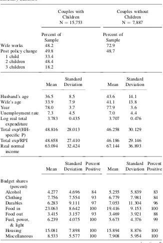
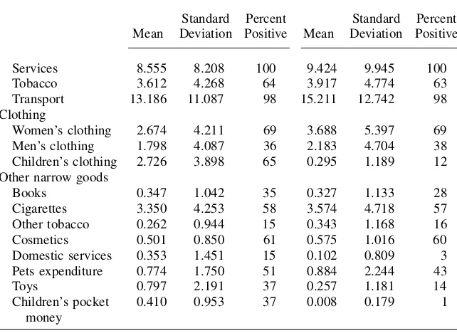
I estimate the model in Equation 1 for 11 broadly defined goods and ten narrowly defined goods, including the three clothing categories, using TSLS. Table 1 presents summary statistics for both with-children and without-children samples, in-cluding means of total expenditure and income measures, and expenditure shares for the goods of interest. The percent of households reporting positive expenditures in each good category is also given. The distribution of families across the three family-size categories is shown for families with children. Almost half of families in the with-chil-dren sample have two chilwith-chil-dren. Thus, the omitted household composition category in estimates is the most common child-age category among two-child families.20
A. Couples with Children
Table 2 presents results for instrumental variable estimates of the 11 broad goods cat-egories.21The three policy-shift variables (for one-, two-, and three-child families)
19. Using log of normal income would require dropping 9 households from the with-children sample and 21 from the no-children sample. However, linear rather than log real normal income is a better predictor of log real total expenditure, so these observations need not be dropped.
20. Frequencies of household composition categories, regions, and quarters of the year are available from the author.
Table 1
Husband’s age 36.5 8.5 43.6 14.1
Wife’s age 33.9 7.9 41.1 13.8
Year 78.0 3.7 77.9 3.6
Unemployment rate 7.3 4.5 7.0 4.4
Log real total
Total exp/RPI 48.658 27.410 46.186 29.146
Real normal
Alcohol 4.277 4.696 84 5.255 5.839 83
Clothing 7.756 7.554 93 6.779 7.981 84
Durables 6.283 9.111 97 7.053 11.304 96
Food in 23.063 8.642 100 19.416 9.153 100
Food out 3.415 3.157 93 3.469 3.921 88
Fuel, power, & light
6.239 4.075 100 5.673 4.376 99
Housing 15.081 7.898 100 15.894 8.876 100
Miscellaneous 8.533 5.577 100 7.908 5.954 100
have a positive and significant effect on expenditure shares for food out and miscel-laneous goods, and negative significant effects on alcohol, food in, and housing. The policy effects on alcohol are negative for all family sizes, and are statistically signif-icant for one- and three-child families. Estimates for broadly defined goods are done equation by equation, and no constraint on adding up of shares is imposed.22F-tests and likelihood-ratio tests were performed for each of the broad goods to test the joint hypothesis that the three policy-shift dummies had no effect. These tests indicate that the policy shift did significantly affect budget shares for alcohol, food in, food out, housing, and miscellaneous goods.
Notes to Table 2 report a chi-square statistic based on a three-stage least squares (3SLS) estimate of the instrumented system of 11 equations, testing the joint hypoth-esis that effects of the three policy variables in all equations are zero.23This hypoth-esis is strongly rejected, indicating that the policy shift did significantly change overall expenditure patterns.
Table 1 (continued)
Mean
Standard Deviation
Percent Positive Mean
Standard Deviation
Percent Positive
Services 8.555 8.208 100 9.424 9.945 100
Tobacco 3.612 4.268 64 3.917 4.774 63
Transport 13.186 11.087 98 15.211 12.742 98
Clothing
Women’s clothing 2.674 4.211 69 3.688 5.397 69
Men’s clothing 1.798 4.087 36 2.183 4.704 38
Children’s clothing 2.726 3.898 65 0.295 1.189 12
Other narrow goods
Books 0.347 1.042 35 0.327 1.133 28
Cigarettes 3.350 4.253 58 3.574 4.718 57
Other tobacco 0.262 0.944 15 0.343 1.168 16
Cosmetics 0.501 0.850 61 0.575 1.016 60
Domestic services 0.353 1.451 15 0.102 0.809 3
Pets expenditure 0.774 1.750 51 0.884 2.244 43
Toys 0.797 2.191 37 0.257 1.181 14
Children’s pocket money
0.410 0.953 37 0.008 0.179 1
Note: Income and expenditure levels are £ per week in 1974 currency.
22. The sum of TSLS policy-change coefficients for budget shares for a given size family is approximately zero, and zero falls near the center of an interval constructed by summing the bottoms and tops of the 11 95 percent confidence intervals.
Table 2
Broad Good Categories—Families with Children, TSLS Estimates of Budget Shares
(1) Alcohol
(2) Clothing
(3) Durables
(4) Food in
(5) Food out
(6) Fuel
(7) Housing
(8) Misc.
(9) Services
(10) Tobacco
(11) Transport
Post policy change
One child -0.642** 0.134 -0.340 -1.794*** 1.212*** 0.367 -2.047*** 0.973*** 0.308 -0.252 0.698 (0.293) (0.460) (0.595) (0.482) (0.236) (0.279) (0.659) (0.340) (0.503) (0.288) (0.682) Two children -0.415 0.398 -0.425 -1.047** 1.051*** 0.278 -2.350*** 0.826** 0.544 -0.166 -0.065
(0.281) (0.442) (0.574) (0.469) (0.229) (0.271) (0.647) (0.327) (0.484) (0.279) (0.656) Three children -0.836*** 0.427 0.112 -1.383*** 0.492** 0.453 -2.421*** 0.938** 0.530 -0.097 0.405
(0.315) (0.496) (0.639) (0.511) (0.249) (0.295) (0.686) (0.368) (0.544) (0.306) (0.737) Ln real total 2.187 22.382***24.313***-38.070***10.983***-32.06*** -6.435 2.449 -44.9*** -23.079***82.443***
expenditure (4.758) (7.524) (9.236) (6.733) (3.227) (3.896) (7.739) (5.625) (8.334) (4.236) (11.255) Ln real -0.202 -2.549***-2.701** 3.049***-1.188*** 3.610*** 0.777 -0.245 6.771*** 2.402***-9.751***
expenditure2 (0.607) (0.960) (1.179) (0.859) (0.412) (0.497) (0.988) (0.718) (1.064) (0.541) (1.437) Ln real 1.175 4.241 7.697 7.433* 1.456 2.371** 9.658***15.147*** 1.537 0.392 3.762
own price (2.351) (2.685) (4.807) (3.854) (1.675) (1.197) (2.477) (3.252) (3.519) (0.996) (6.439) R2 0.0472 0.0800 0.0469 0.4366 0.0300 0.1517 0.1097 0.0556 0.0419 0.0865 0.0448 F 3.01** 0.60 0.74 6.27*** 15.18*** 0.94 4.78*** 2.86** 0.57 0.39 1.37
Note: N¼15,753. Standard errors in parentheses. Estimates include a constant, age of both spouses, household composition category (children’s ages), region, unem-ployment rate, quarter of the year, and quadratic time trend. * Significant at 10 percent; ** Significant at 5 percent; *** Significant at 1 percent. Cross-equation joint hypothesis test that all policy variables¼0:x2
(33)¼130.04*** using 3SLS or 129.54*** using a two-step SUR procedure.Fstatistic is for the joint hypothesis that all three policy variables have no effect.
The
Journal
of
Human
Phipps and Burton (1998) and Hoddinott and Haddad (1995) find negative effects of the wife’s relative income on tobacco and alcohol; Attanasio and Lechene (2002) find negative effects of the wife’s relative income on alcohol. I find negative effects here of the Child Benefit policy change on alcohol. The sign on tobacco is negative, but these effects are not significant. Phipps and Burton also found positive effects of the wife’s income on restaurant meals. This could be interpreted as a price effect since the study uses earned income as the key explanatory variable. The exogeneity of the policy change in the present analysis rules out such an interpretation here of the strong pos-itive effect on ‘‘food out,’’ which includes restaurant meals and take-away food, and the negative effect on food in. These results suggest a substitution of more restaurant and take-away meals for the mother’s time in preparing food at home.
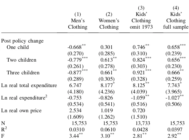
Table 3 reports results from expenditure share equations on the narrow clothing categories examined by LPW.24I find significant declines in the budget share for men’s clothing in all family sizes, and increases in women’s clothing that are signif-icant in two- and three-child families. Children’s clothing estimates in Columns 3 and 4 indicate a strongly significant increase in their budget share associated with the policy change. The children’s clothing price index is only available from 1974. Thus, Column 3 estimates omit data for 1973 in order to include price in the model, while Column 4 uses all of the data, but omits price.
These results confirm those found by LPW, and suggest that the increase in the ratio of women’s to men’s clothing is driven by changes in both, but perhaps more to declines in men’s than to increases in women’s clothing, given the relatively larger effects I find on the former. This is important, as some critics have speculated that the change in that ratio may have been driven by increased labor force participation of women over the period (and consequent greater expenditure on their clothing), rather than by this policy change shifting control of income—a point I will return to. It is also clear from estimates here that the ratio of children’s to men’s clothing will have risen due to significant changes in both goods, and that changes in this ratio were not solely attributable to coincident changes in VAT rates.25 These results strengthen the case that these shifts in expenditures are attributable in part to the Child Benefit policy change and the apparent preference of mothers to allocate more of the family budget to children’s goods.
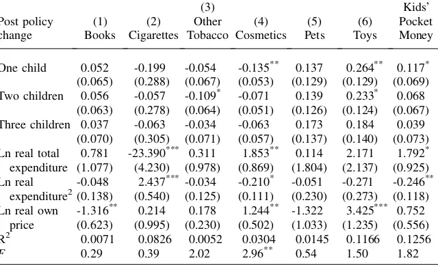
Budget shares for seven additional narrowly defined goods are estimated: books, cigarettes, other tobacco, cosmetics, pets expenditures, toys, and children’s pocket money. These goods are of interest either because they may be of greater interest to certain household members (men, women, or children), or because their consump-tion may have some impact on child well-being or development (for example, books). Results appear in Table 4.
Cigarettes expenditures do not appear to have been significantly affected by the policy change, though coefficients are consistently negative, but other tobacco expen-ditures show a marginally significant decline for two-child families. Separating the two categories is potentially interesting because, while both men and women
24. These clothing categories include footwear. The three narrow clothing shares may not sum to the over-all clothing share due to a smover-all fraction of the total being unassignable in nature.
commonly consume cigarettes, the ‘‘other tobacco’’ category comprises goods pri-marily consumed by men during the period examined. Nevertheless, tobacco prod-ucts generally are included among the vices that studies of intrahousehold resource allocation often examine.
There are no significant effects on books or pets expenditures. Cosmetics expen-ditures declined significantly for one-child families. The policy effects on toys and pocket money are all positive. These are significant for toys in one- and two-child families, and for children’s pocket money in one-child families. These results pro-vide further epro-vidence that children’s goods increased in the budget when the policy change reallocated income from fathers to mothers.
The magnitudes of changes in budget shares these results suggest are certainly plausible given the amount of income being shifted from men to women. For in-stance, for the average two-child family the change in expenditures on the broad cat-egory ‘‘food out’’ due to the policy change is about £27 per year. The same family decreased its annual ‘‘food in’’ expenditure by £26, decreased housing expenditure by £59, and increased children’s clothing expenditures by £21 and toys expenditures by £6. The average annual changes in men’s and women’s clothing expenditures is Table 3
TSLS Estimates of Clothing Budget Shares—Families with Children
(1)
Ln real total expenditure 6.747 8.177* 8.125** 7.743*
(4.180) (4.236) (4.039) (3.965)
Ln real expenditure2 -0.753 -0.826 -1.059** -1.027**
(0.534) (0.541) (0.516) (0.506)
Ln real own price 2.534 1.019 0.720
(1.609) (1.262) (1.510)
N 15,753 15,753 13,733 15,753
R2 0.0310 0.0610 0.0428 0.0397
F 3.44** 3.10** 2.81** 2.92**
-£21 and £16 respectively. These are reasonable magnitudes given that £134 per year or more was shifted from husband to wife.26
Bradbury (2004) does not find evidence against income pooling in Australian data when income is similarly reallocated in income families. He speculates that low-income households may behave differently. To check for this in the United Kingdom data, I reestimate all of my models using only households below the median total expenditure for the year in which they are surveyed (results available from the au-thor). I find the negative effect on alcohol is about the same magnitude for three-child families as in the full sample, but is only significant at 10 percent, due in part to the smaller sample. The effect on alcohol is smaller for one- and two-child families, and is not significant. Coefficients for the aggregate clothing category are much larger than in the full sample, and are significant at 5 percent or 1 percent depending on family size. Effects on food-in are not significant, and some coefficients become pos-itive, but effects on food out are pospos-itive, and are significant at 1 percent for one-and two-child families. Effects on housing one-and miscellaneous goods are larger in magnitude than in the full sample, and significant at 1 percent for all family sizes. Table 4
Narrowly Defined Goods, Families with Children, TSLS
Post policy
One child 0.052 -0.199 -0.054 -0.135** 0.137 0.264** 0.117* (0.065) (0.288) (0.067) (0.053) (0.129) (0.129) (0.069) Two children 0.056 -0.057 -0.109* -0.071 0.139 0.233* 0.068
(0.063) (0.278) (0.064) (0.051) (0.126) (0.124) (0.067) Three children 0.037 -0.063 -0.034 -0.063 0.173 0.184 0.039
(0.070) (0.305) (0.071) (0.057) (0.137) (0.140) (0.073) Ln real total 0.781 -23.390*** 0.311 1.853** 0.114 2.171 1.792* expenditure (1.077) (4.230) (0.978) (0.869) (1.804) (2.137) (0.925) Ln real -0.048 2.437*** -0.034 -0.210* -0.051 -0.271 -0.246**
expenditure2(0.138) (0.540) (0.125) (0.111) (0.230) (0.273) (0.118) Ln real own -1.316** 0.214 0.178 1.244** -1.322 3.425*** 0.752
price (0.623) (0.995) (0.230) (0.502) (1.033) (1.235) (0.556)
R2 0.0071 0.0826 0.0052 0.0304 0.0145 0.1166 0.1256
F 0.29 0.39 2.02 2.96** 0.54 1.50 1.82
Note: N¼15,753. Standard errors in parentheses. Estimates include a constant, age of both spouses, house-hold composition category (based on number of children and their ages), region, unemployment rate, quar-ter of the year, and quadratic time trend.F-statistic is for the joint hypothesis that all three policy variables have no effect. Model 7 controls for miscellaneous price (shown) and food out price (not shown). * Signif-icant at 10 percent; ** SignifSignif-icant at 5 percent; *** SignifSignif-icant at 1 percent.
Coefficients for tobacco are positive in this group, opposite from the full sample, but are not statistically significant. Effects on men’s clothing results are near zero and not significant, but positive effects on women’s clothing remain significant for two- and three-child families. Children’s clothing results are larger in magnitude with signif-icance levels similar to the full sample. Coefficients are consistently negative for cos-metics and positive for children’s pocket money, but neither is significant. The effect on toys is slightly larger than in the full sample, and significant at 10 percent for one-child families. In general, results for the below-median-expenditure sample look sim-ilar to, but somewhat weaker than, those for the full sample.
B. Couples Without Children
The ‘‘natural experiment’’ exploited here is imperfect in that there is no control group randomly assigned to not receive the treatment. It is plausible that the effects reported thus far are due to secular shifts in expenditures that are not captured by the quadratic time trend, and that they are not caused by the redistribution of income within the fam-ily. As Hotchkiss (2005) rightly points out, it is important to verify that similar ‘‘effects’’ do not occur in an untreated group. Therefore, I check whether similar shifts may be found among couples in households with no children.27These may consist of couples who will never have children, those who will but have not yet had children, and those whose children are now adults that have moved away from the parental house-hold. One could argue that the policy may have some effect on those who plan to later have children, as it shifts some of the couple’s expected permanent income from the husband to the wife. If this effect exists, it is likely small relative to the effect we should expect among families currently receiving the benefit, and smaller still in the untreated group as a whole, given that these households make up only a fraction of that group. With the exception of exclusive children’s goods, the same expenditure shares as above are estimated for married-couple households with no children.28Table 5 shows TSLS estimates of the 11 broadly defined goods for couples without children. A sin-gle dummy variable is used to represent the post-policy-change period. The policy does not significantly affect expenditures in any of the categories, and the null hy-pothesis fails to be rejected in a joint test across the 11 equations. Table 6 shows esti-mates of men’s and women’s clothing shares in the first two columns. There are no significant ‘‘effects’’ of the policy, and coefficients are opposite in sign to those in families with children. Columns 3–8 of Table 6 show estimates of the remaining nar-row goods. The only goods with significant effects of the policy dummy are among the tobacco categories. A positive effect on cigarettes is significant at 10 percent. This is opposite in sign from coefficients for families with children. I find a negative significant effect here on other tobacco. This casts doubt on the decline in this men’s good among families with children being solely attributable to the policy change. A separate price index for cigarettes versus other tobacco is not available. It is plau-sible that there are relative price changes between these two goods over this period that are not adequately controlled for in these estimates. For the vast majority of
27. As in those with children, these couples may be married, or unmarried but living as husband and wife. I refer to them as married couples for convenience.
(1) Alcohol
(2) Clothing
(3) Durables
(4) Food in
(5) Food out
(6) Fuel
(7) Housing
(8) Misc.
(9) Services
(10) Tobacco
(11) Transport
Post policy -0.159 0.686 0.229 0.182 -0.258 0.551 -1.187 0.376 -0.758 0.520 0.048
change (0.485) (0.644) (0.980) (0.646) (0.391) (0.396) (1.032) (0.489) (0.787) (0.428) (1.019)
Ln real total -3.226 20.475 23.862 -50.14*** 7.544 -21.6*** -35.3** -8.444 -3.033 -16.39** 85.65***
expenditure (10.085) (13.497) (19.187) (11.429) (6.701) (6.926) (15.072) (10.414) (16.749) (7.999) (21.63)
Ln real expenditure2 0.462 -2.429 -2.654 4.85*** -0.691 2.38*** 4.502** 1.037 1.473 1.571 -10.42***
(1.321) (1.768) (2.513) (1.497) (0.878) (0.907) (1.974) (1.364) (2.194) (1.048) (2.833)
Ln real own -0.712 1.605 2.952 4.377 -3.893 4.352** 5.279 6.220 -0.074 2.095 -6.657
price (4.134) (4.035) (8.338) (5.448) (2.936) (1.783) (4.066) (5.066) (5.860) (1.580) (10.418)
R2 0.0344 0.0707 0.0638 0.4960 0.0508 0.1893 0.0603 0.0086 0.0791 0.0893 0.0651
Note: N¼7,887. Standard errors in parentheses. Estimates include a constant, age of both spouses, region, unemployment rate, quarter of the year, and quadratic time trend. Cross-equation joint hypothesis test that policy variable¼0:x2(11)¼3.78 using 3SLS or 7.43 using a two-step SUR procedure. * Significant at 10 percent;
** Significant at 5 percent; *** Significant at 1 percent.
W
ard-Batts
Table 6
TSLS Clothing and Other Narrow Goods, Budget Shares—Couples with No Children
(1) Men’s Clothing
(2) Women’s Clothing
(3) Books
(4) Cigarettes
(5) Other Tobacco
(6) Cosmetics
(7) Pets
(8) Toys
Post policy change 0.456 -0.107 -0.075 0.772* -0.252** -0.030 0.098 0.048
(0.415) (0.490) (0.095) (0.426) (0.109) (0.082) (0.224) (0.096)
Ln real total expenditure 11.101 5.460 -4.710** -18.758** 2.373 1.797 -6.661* 0.076
(8.136) (9.258) (2.028) (7.965) (2.037) (1.756) (3.960) (2.046)
Ln expenditure squared -1.347 -0.569 0.644** 1.882* -0.311 -0.220 0.810 -0.034
(1.066) (1.212) (0.266) (1.043) (0.267) (0.230) (0.519) (0.268)
Ln real own price 1.631 -1.170 -0.709 2.355 -0.260 0.981 -0.996 -0.064
(2.629) (2.297) (0.987) (1.573) (0.402) (0.854) (1.887) (0.995)
R2 0.0282 0.0424 0.0204a 0.0755 0.0123 0.0325 0.0103a 0.0273
Note: N¼7,887. Standard errors in parentheses. Estimates include a constant, age of both spouses, region, unemployment rate, quarter of the year, and quadratic time trend. * Significant at 10 percent; ** Significant at 5 percent; *** Significant at 1 percent.
a. R2not estimated in TSLS. That from OLS model shown.
The
Journal
of
Human
goods examined, there is no evidence that married-couple households with no chil-dren, the untreated group, changed their behavior in a similar way as couples with children around the time of this policy change.
In some cases, the contrast between couples with and without children indicates potentially larger effects of the policy than it first appeared. For example, if there was a secular increase in consumption of cigarettes overall, but we do not see that in couples with children, then it may be the shifting of income control that prevented those households from increasing their expenditures on cigarettes.
This control group is not a good candidate for use in a traditional difference-in-dif-ference estimator. Pooling the treated and untreated groups for the period 1973–76, I cannot reject the null hypothesis that the time trends in expenditures differ between the two groups in the prepolicy-change period. Nevertheless, I pool the groups and estimate a fully interacted model for the entire period, allowing all parameters to dif-fer for the two groups. I estimate the difdif-ference in the average effect for families with children and the effect for households with no children. This difference for each of the relevant goods categories is reported in Table A3 in the appendix.
C. Robustness Checks
Even in a unitary model, a secular increase in women’s labor supply over the period examined could be an alternate explanation for the expenditure shifts found here in some goods, such as women’s clothing, and food in and out. Because women’s labor supply is endogenously determined with household expenditures, controlling for it in expenditure estimates is problematic. Gray (1998) finds that married women’s labor supply in the United States increases when their bargaining power increases due to changes in marital property laws, even when controlling for changes in divorce law. In spite of the concern about endogeneity of the wife’s labor supply, I reestimate all of the expenditure estimates herein while controlling for whether the wife works. This variable is significant for some goods, but the estimated impacts of the Child Benefit policy change are unaffected (results available from the author).
Another concern is that the treatment group sample is approximately twice the size of the untreated sample. To check what impact the smaller sample size has on sig-nificance levels, I duplicate the untreated group, doubling its size, and reestimate all of the expenditure equations. The coefficients are obviously the same as those reported herein. The ‘‘effect’’ of the post-policy dummy becomes significant for fuel at 5 percent and for tobacco at 10 percent. The significance for cigarettes changes from 10 percent to 5 percent, and for other tobacco from 5 percent to 1 percent. The policy variable is not significant for any of the other goods.
tobit and probit models, but we also see a significant decline in the control group in these models. If there is a secular decrease over the period not captured by time trends, then the effects on cosmetics among the treatment group may not be due to the shift in intra-household income distribution. We also see more significant ‘‘effects’’ on cigarettes for families without children as in the TSLS estimates, but neither cigarettes nor other to-bacco is significant in families with children. If the price of cigarettes fell relative to other tobacco over the period, this could explain what appears to be a substitution of the former for the latter among households without children. This shift does not appear to have occurred among families with children.
VI. Conclusion
I use household-level data to examine how budget shares changed in two-parent families with children in the United Kingdom when a change in Family Allowance policy shifted transfer income from fathers to mothers. Shifts in expendi-ture patterns due to this change are inconsistent with the unitary model of household decisions. The results reported here support results in Lundberg, Pollak, and Wales (1997) rejecting income pooling, and address concerns of Hotchkiss (2005) that an untreated group should also be examined.
I find significant changes in expenditures on broadly defined goods, as well as on some narrowly defined goods which may be of greater interest to men, women, or children. Although we may not have strong priors about the direction of change for all of the broad goods categories, the discrete change found in shares in the before versus after period which is not attributable to other factors indicates that there has been a shift of power over decision making in the household, and that a systematic difference in preferences over allocation of household income exists between husbands and wives. Closer examination of expenditures on select goods among and within these broad cat-egories produces further insights. These shifts indicate that women and children benefited at the expense of men when this new policy took effect.
Alcohol and men’s clothing decreased in the budget, while women’s and children’s clothing, toys, and children’s pocket money increased as a share of expenditure. A decrease in expenditures on food for home preparation coupled with an increase in expenditures on restaurant meals and take-away food suggest a decline in home production effort of wives and greater reliance on market-produced substitutes.
Estimates of budget shares among married-couple households with no children do not show a similar pattern of change to that in households with children. The sample without children shows no change in broad goods expenditures, or in narrowly defined goods with the exception of tobacco categories. A marginally significant increase in cigarettes is op-posite in sign to point estimates in households with children. Other tobacco is the only good for which similar changes are found in households with and without children.
household members—any reallocation of resources within the household will be un-done by the household. To the contrary, these results suggest that transfers targeted at particular household members can be effective.
Appendix 1
Table A1
Example of First Stage for Expenditure Share Estimates—Couples with Children
Log real total expenditure
Square of log real total expenditure
(1) (2) (3) (4) (5) (6)
Real normal income 0.011*** 0.011*** 0.087*** 0.081***
(0.000) (0.000) (0.001) (0.001)
Real normal income2 -0.000*** -0.000*** -0.000*** -0.000***
(0.000) (0.000) (0.000) (0.000)
Ln real price 0.372* 0.331 2.775* 2.471
(0.206) (0.246) (1.630) (1.943)
Head age 0.001 0.000 0.006 0.006***
(0.001) (0.001) (0.006) (0.007)
Wife age 0.003*** 0.009*** 0.018*** 0.070
(0.001) (0.001) (0.006) (0.008)
Year -0.033*** -0.030*** -0.248*** -0.228***
(0.006) (0.007) (0.044) (0.052)
Year2 0.002*** 0.003*** 0.016*** 0.024***
(0.000) (0.000) (0.003) (0.004)
Unemployment rate -0.002 -0.012*** -0.011 -0.089***
(0.003) (0.003) (0.021) (0.025)
Post-change X 3.143*** 3.805*** 4.208*** 9.582*** 14.758** 17.805** one child (0.008) (0.882) (1.055) (0.064) (6.992) (8.336) Post-change X 0.011*** 0.011*** 0.087*** 0.081***
two children (0.000) (0.000) (0.001) (0.001)
Post-change X -0.000*** -0.000*** -0.000*** -0.000*** three children (0.000) (0.000) (0.000) (0.000)
Constant 0.372* 0.331 2.775* 2.471
(0.206) (0.246) (1.630) (1.943)
F 3394.5*** 3314.6***
R2 0.3529 0.3785 0.1101 0.3466 0.3698 0.1040
Adjusted R2 0.3528 0.3772 0.1083 0.3465 0.3684 0.1022
Table A2
Example of First Stage for Expenditure Share Estimates—Couples without Children
Log real total expenditure
Square of log real total expenditure
(1) (2) (3) (4) (5) (6)
Real normal 0.011*** 0.011*** 0.081*** 0.079***
income (0.000) (0.000) (0.002) (0.002)
Real normal -0.000*** -0.000*** -0.000*** -0.000***
income2 (0.000) (0.000) (0.000) (0.000)
Log real price miscellaneous goods
0.380 0.398 2.520 2.644
(0.330) (0.394) (2.573) (3.048)
Post change 0.112*** 0.108*** 0.833*** 0.811***
(0.032) (0.038) (0.249) (0.295)
Year -0.053***-0.039*** -0.403*** -0.299***
(0.009) (0.010) (0.068) (0.081)
Year2 0.003*** 0.003*** 0.023*** 0.026***
(0.001) (0.001) (0.005) (0.006)
Head age 0.001 -0.002 0.013 -0.010
(0.001) (0.001) (0.008) (0.010)
Wife age -0.002 -0.002 -0.012 -0.013
(0.001) (0.001) (0.009) (0.010)
Unemployment 0.001 -0.011** 0.007 -0.080**
rate (0.004) (0.005) (0.034) (0.040)
Constant 3.069*** 5.280*** 5.001*** 9.159*** 27.288** 25.358* (0.012) (1.411) (1.682) (0.092) (10.994) (13.026)
F 1,655.12*** 1,589.69***
R2 0.3212 0.3342 0.0539 0.3111 0.3234 0.0499
Adjusted R2 0.3211 0.3323 0.0514 0.3109 0.3214 0.0473
Panel A: Broad Goods
Alcohol Clothing Durables Food in Food out Fuel Housing Miscellaneous Services Tobacco Transport
-0.398 -0.366 -0.541 -1.522* 1.263*** -0.216 -1.079 0.515 1.225 -0.700 0.208
(0.516) (0.757) (1.052) (0.791) (0.421) (0.468) (1.156) (0.565) (0.864) (0.489) (1.150)"
Panel B: Narrow Goods
Men’s Clothing Women’s Clothing Books Cigarettes Other Tobacco Cosmetics Pets Toys
-1.217*** 0.626 0.126 -0.873* 0.173 -0.060 0.046 0.187
(0.464) (0.515) (0.109) (0.488) (0.117) (0.090) (0.235) (0.183)
Note: N¼23,640. Standard errors in parentheses. Estimates include all control variables included in estimates reported in Tables 2-6, interacted with a dummy for the sample with children where appropriate. * Significant at 10 percent; ** Significant at 5 percent; *** Significant at 1 percent.
W
ard-Batts
Table A4
Instrumental Variable Tobits and Probits for Select Goods
Panel A: IV Tobits, Families with Children (N¼15,753)
Post policy change: Alcohol Tobacco Food out Cigarettes Other tobacco Cosmetics Pets KidsÕpocket money
One child -0.781** -0.258 1.349*** -0.204 -0.305 -0.328*** 0.344 0.288*
(0.342) (0.431) (0.251) (0.473) (0.374) (0.081) (0.232) (0.167)
Two children -0.484 -0.190 1.165*** -0.069 -0.522 -0.257*** 0.278 0.250
(0.329) (0.417) (0.244) (0.458) (0.360) (0.078) (0.225) (0.159)
Three children -0.936** -0.024 0.564** 0.034 -0.133 -0.239*** 0.347 0.244
(0.369) (0.457) (0.264) (0.502) (0.399) (0.088) (0.245) (0.168)
Chi sq(3) 8.73** 0.89 48.59*** 0.69 4.38 16.74*** 2.44 2.99
Panel B: IV Probits, Families with Children (N¼15,753)
One child -0.024 -0.037 0.042*** -0.013 -0.021 -0.154*** 0.052 0.081*
(0.036) (0.025) (0.008) (0.036) (0.024) (0.032) (0.038) (0.042)
Two children -0.022 -0.023 0.042*** -0.014 -0.031 -0.152*** 0.031 0.065
(0.034) (0.023) (0.010) (0.035) (0.023) (0.031) (0.037) (0.039)
Three children -0.009 -0.028 0.027*** -0.002 -0.009 -0.135*** 0.042 0.052
(0.037) (0.027) (0.010) (0.038) (0.026) (0.035) (0.040) (0.043)
Chi sq(3) 0.81 2.51 18.31*** 0.39 3.35 26.53*** 2.52 4.52
(continued)
The
Journal
of
Human
Panel C: IV Tobits, Families without Children (N¼7,887)
Post policy change -0.018 0.846 -0.143 1.722** -1.395** -0.275** 0.047 (0.570) (0.646) (0.435) (0.717) (0.613) (0.129) (0.458)
Panel D: IV Probits, Families without Children (N¼7,887)
Post policy change 0.042 0.040 0.047* 0.126*** -0.067** -0.173*** -0.014 (0.031) (0.047) (0.028) (0.048) (0.034) (0.040) (0.050)
Note: Probit marginal effects are reported. Standard errors in parentheses. Estimates includes a constant, age of both spouses, household composition category (chindren’s ages), region unemployment rate, quarter of the year, and quadratic time trend, log real own price and a quadratic in log real total expenditure. Chi-square statistic is for the joint hypothesis that all three policy variables have no effect.
*Significant at 10 present; **Significant at 5 percent; ***Significant 1 percent
W
ard-Batts
References
Attanasio, Orazio, and Vale´rie Lechene. 2002. ‘‘Tests of Income Pooling in Household Decisions.’’Review of Economic Dynamics5(4):720–48.
Banks, James, Richard Blundell, and Sarah Tanner. 1998. ‘‘Is There a Retirement Savings Puzzle?’’American Economic Review88(4):769–88.
Banks, James, Richard Blundell, and Arthur Lewbel. 1997. ‘‘Quadratic Engel Curves and Consumer Demand.’’Review of Economics and Statistics79(4):527–39.
Becker, Gary. 1981.A Treatise on the Family. Cambridge, Mass.: Harvard University Press. Bergstrom, Theodore. 1996. ‘‘A Survey of Theories of the Family.’’ InHandbook of
Population and Family Economics1A, ed. Mark R. Rosenzweig and Oded Stark, 21–79. Amsterdam; New York and Oxford: Elsevier Science, North-Holland.
Bingley, Paul, and Ian Walker. 1997. ‘‘There is No Such Thing as a Free Lunch: Evidence from the Effect of In-Kind Transfers.’’ Institute for Fiscal Studies, IFS Working Papers: W97/07.
Blundell, Richard, and Costas Meghir. 1987. ‘‘Bivariate Alternatives to the Tobit Model.’’ Journal of Econometrics34(2):179–200.
Bourguinon, Francois, Martin Browning, Pierre-Andre Chiappori, and Vale´rie Lechene. 1993. ‘‘Intra Household Allocation of Consumption: A Model and Some Evidence from French Data.’’Annales d’Economie et de Statistique0(29):137–56.
Bradbury, Bruce. 2004. ‘‘Consumption and the Within-Household Income Distribution: Outcomes from an AustralianÔNatural ExperimentÕ.’’CESifo Economic Studies50(3):501– 40.
Central Statistical Office. 1984–87.Annual Abstract of Statistics. London: HMSO. Chiappori, Pierre-Andre. 1988. ‘‘Rational Household Labor Supply.’’Econometrica
56(1):63–90.
———. 1992. ‘‘Collective Labor Supply and Welfare.’’Journal of Political Economy 100(3):437–67.
Cragg, John G. 1971. ‘‘Some Statistical Models for Limited Dependent Variables with Application to the Demand for Durable Goods. ’’Econometrica39(5):829–844. Deaton, Angus, and John Muellbauer. 1980a. ‘‘An Almost Ideal Demand System.’’American
Economic Review70(3):312–26.
———. 1980b.Economics and Consumer Behavior. New York: Cambridge University Press. Department of Employment and Productivity. 1973–76, 1980–83.Family Expenditure Survey.
London: HMSO.
Department of Health and Social Security. 1991.Social Security Statistics. London: HMSO. Duflo, Esther. 2003. ‘‘Grandmothers and Granddaughters: Old-Age Pensions and
Intrahousehold Allocation in South Africa.’’The World Bank Economic Review17(1):1–25. Edmonds, Eric. 2002. ‘‘Reconsidering the Labeling Effect for Child Benefits: Evidence from
a Transition Economy.’’Economics Letters76:303–309.
Gray, Jeffrey. 1998. ‘‘Divorce-Law Changes, Household Bargaining, and Married Women’s Labor Supply.’’American Economic Review88(3):628–42.
Hoddinott, John and Lawrence Haddad. 1995. ‘‘Does Female Income Share Influence Household Expenditures: Evidence from The Cote d’Ivoire.’’Oxford Bulletin of Economics and Statistics57(1):77–96.
Hotchkiss, Julie L. 2005. ‘‘Do Husbands and Wives Pool Their Resources? Further Evidence,’’Journal of Human Resources40(2):519–31.
House of Commons. 1975.Hansard. May, London: HMSO.
Keen, Michael. 1986. ‘‘Zero Expenditures and the Estimation of Engel Curves.’’Journal of Applied Econometrics1(3):277–86.
Kooreman, Peter. 2000. ‘‘The Labeling Effect of a Child Benefit System.’’American Economic Review90(3):571–83.
Lundberg, Shelly J. 1999. ‘‘Family Bargaining and Retirement Behavior.’’ InBehavioral Dimensions of Retirement Economics, ed. Henry Aaron, 253–72. Washington, D.C.: Brookings Institution Press. New York: Russell Sage Foundation.
Lundberg, Shelly J., and Robert A. Pollak. 1993. ‘‘Separate Spheres Bargaining and the Marriage Market.’’Journal of Political Economy101(6):988–1010.
———. 1994. ‘‘Noncooperative Bargaining Models of Marriage.’’American Economic Review84(2):132–37.
———. 1996. ‘‘Bargaining and Distribution in Marriage.’’Journal of Economic Perspectives 10(4):139–58.
Lundberg, Shelly J., Robert A. Pollak, and Terry J. Wales. 1997. ‘‘Do Husbands and Wives Pool Their Resources? Evidence from the U.K. Child Benefit.’’Journal of Human Resources32(3):463–80.
Lundberg, Shelly J., Richard Startz, and Steven Stillman. 2003. ‘‘The Retirement-Consumption Puzzle: A Marital Bargaining Approach.’’Journal of Public Economics 87(5–6):1199–1218.
Manser, Marilyn, and Murray Brown. 1980. ‘‘Marriage and Household Decision Making: A Bargaining Analysis.’’International Economic Review21(1):31–44.
McElroy, Marjorie B., and Mary Jean Horney. 1981. ‘‘Nash Bargained Household Decisions.’’ International Economic Review22(2):333–49.
Moehling, Carolyn. 2003. ‘‘The Incentives to Work: Working Children and Household Decision-Making.’’ Unpublished.
Phipps, Shelley, and Peter Burton. 1998. ‘‘What’s Mine is Yours? The Influence of Male and Female Incomes on Patterns of Household Expenditure.’’Economica65(260):599–613. Prest, A.R. 1980.Value Added Taxation: The Experience of the United Kingdom. Washington:
American Enterprise Institute for Public Policy Research.
Quisumbing, Agnes R., and John. A. Maluccio. 2003. ‘‘Resources at Marriage and Intrahousehold Allocation: Evidence from Bangladesh, Ethiopia, Indonesia, and South Africa.’’Oxford Bulletin of Economics and Statistics65(3):283–328.
Samuelson, Paul A. 1956. ‘‘Social Indifference Curves.’’Quarterly Journal of Economics 70(1):1–22.
Schultz, T. Paul. 1990. ‘‘Testing the Neoclassical Model of Family Labor Supply and Fertility.’’Journal of Human Resources25(4):599–634.
Thomas, Duncan. 1990. ‘‘Intra-household Resource Allocation: An Inferential Approach.’’ Journal of Human Resources25(4):635–64.