Michael Insler is an assistant professor of economics at the United States Naval Academy. He is very grate-ful to Ronni Pavan for extraordinary help and guidance, as well as Mark Bils, Gregorio Caetano, Joshua Kinsler, Nese Yildiz, and the students and faculty at the University of Rochester Applied / Macro lunch seminar for their useful suggestions. He also thanks two anonymous referees for many helpful remarks. Researchers may acquire the data used in this article from RAND’s Center for the Study of Aging (http: // www .rand .org / labor / aging / dataprod / hrs- data .html). For questions regarding the data, please contact Michael Insler, insler@usna .edu.
ISSN 0022- 166X E- ISSN 1548- 8004 © 2014 by the Board of Regents of the University of Wisconsin System
T H E J O U R N A L O F H U M A N R E S O U R C E S • 49 • 1
of Retirement
Michael Insler
A B S T R A C T
This paper examines the impact of retirement on individuals’ health. Declines in health commonly compel workers to retire, so the challenge is to disentangle the simultaneous causal effects. The estimation strategy employs an instrumental variables specifi cation. The instrument is based on workers’ self- reported probabilities of working past ages 62 and 65, taken from the fi rst period in which they are observed. Results indicate that the retirement effect on health is benefi cial and signifi cant. Investigation into behavioral data, such as smoking and exercise, suggests that retirement may affect health through such channels. With additional leisure time, many retirees practice healthier habits.
I. Introduction
us-age. This paper estimates the causal impact of retirement on health. A more complete understanding of the health consequences of retirement will provide a better notion of the economic impact of potential changes to Social Security and Medicare. In general, this new information will allow economists to forecast payout and tax streams more accurately and to model healthcare needs, insurance plans, and labor market transi-tions with more precision.
A. Background
There is a well- established connection between health and work. Numerous studies have researched the relationship between health and labor supply, a topic that is closely associated with the health insurance market. For many workers, the role of private health insurance can be an important part of their labor market decisions. For instance, there is strong evidence that health insurance is a major factor in the labor force partic-ipation of secondary wage earners: Several studies have estimated that spouse- covered health insurance reduces own- labor force participation by seven to 11 percentage points.1 Most relevant to the current study, however, is the substantial evidence that
health insurance is an integral component of workers’ retirement decisions. Gustman and Steinmeier (1994) found that employer provision of retiree health insurance delays retirement until the eligibility age for such coverage and accelerates it thereafter. Rust and Phelan (1997) determined that, due to the Medicare eligibility age of 65, men with employer- provided health insurance but without employer- provided health coverage in retirement are less likely to retire before age 65 than those with health insurance that spans retirement. Moreover, if it is true that the strong link between expansive public policies and retirement behavior stems not only from health insurance but also from health status, then the latter connection also merits close scrutiny.
Many studies have examined the “retirement- health nexus,” particularly the role of health status in individuals’ retirement decisions. Anderson and Burkhauser (1985) posed the question of whether retirement plans are driven by economic variables as much as by health. Although their results differed depending on the choice of health measure (self- reported health or mortality), they found that self- assessed health effects on retirement were larger than wage effects. Bazzoli (1985) compared preretirement and postretirement health information, concluding (oppositely) that economic factors, rather than health, had the larger infl uence on retirement decisions.2 Dwyer and
Mitch-ell (1999) utilized more detailed, longitudinal health data to argue that health indeed plays a major role in retirement. McGarry (2004) developed a model to examine the effect of health on retirement expectations, concluding that health has a much larger impact than economic factors on the probability of working. This literature reveals that the health- retirement simultaneity issue is pervasive, and an important converse question remains on how retirement may infl uence health.3
What are the implications of retirement’s effect on health, should it exist? As stated earlier, there may be second- order effects. Rust and Phelan (1997) indicated that
1. Olson (1998); Buchmueller and Valletta (1999).
2. Bazzoli’s results, like those of Anderson and Burkhauser (1985) stemming from mortality, may have been impacted by poorly measured health variables in the data.
changes to Social Security and Medicare would infl uence retirement behavior, but it remains unknown whether subsequent retirement- driven health changes (if they exist) could in turn affect the fi nances of those programs. Is there any evidence, a priori, that such second- order effects may be signifi cant and hence worth investigating? In 2002, individuals age 65 and over comprised 13 percent of the U.S. population, but they consumed 36 percent of total U.S. personal healthcare expenses (Stanton 2006). Thus it is clear that factors affecting late- career workers’ and retirees’ health are of great
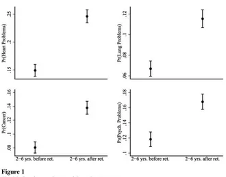
fi scal importance, particularly with respect to discussions regarding the long- term viability of Medicare. Moreover, the fi ve most expensive health conditions in 2002 were heart disease, cancer, trauma, psychological disorders, and pulmonary conditions (Olin and Rhoades 2006). Four of those fi ve conditions (all but trauma) are captured by the health metrics used throughout this paper, and 2002 is near the midpoint of the longitudinal data employed by the main empirical work to come. Figure 1 presents sample proportions and 95 percent confi dence intervals for those four conditions (data is from the main sample, which will be described in Section III). Most notably, there is a large and statistically signifi cant increase in the incidence of each ailment, transition-ing from late- career workers to recent retirees, jumptransition-ing by as much as ten percentage points in the case of heart problems. These simple correlations illustrate a potential pitfall of not carefully examining the health consequences of retirement. Without a Figure 1
Health Conditions Pre- and Post- Retirement
thorough investigation, basic analysis might lead one to believe that retirement exac-erbates the most costly and pervasive health conditions, whereas the main results of Section V will show that, in fact, the opposite is true. Such fallacious reasoning could lead to uninformed policy recommendations or poor budgetary projections, potentially harmful to important aspects of fi scal policy, including Medicare, Social Security, and other programs.
B. Framework
In examining this question, the challenge is to properly treat the simultaneous effects that may cloud the true impact of retirement on health. In particular, it is common for workers to retire when they become ill or injured, and as a result, poor health may bring about retirement.4 There is no strong consensus regarding the converse effect,
which may operate in different directions.5 On the one hand, retirement may lead to
a negative lifestyle shock, a loss of ambition, or a general decrease in activity level, expediting the decline in health that naturally accompanies aging. On the other hand, retirement provides retirees with more leisure time so they may address their “health upkeep” needs and experience less job- related stress and strain. This paper constructs an econometric model that allows estimation of retirement’s net effect on individuals’ health.
Simple empirical analysis of data from the Health and Retirement Study (HRS) sug-gests that simultaneous effects are indeed present.6 In this paper, it is crucial to
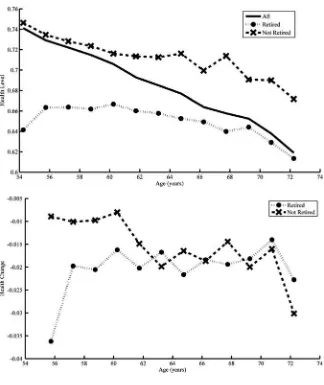
prop-erly measure and interpret the notion of “general health.” Section III provides details on the health metrics, but for now, let health be measured by a univariate scale from zero to one. Figure 2 contains sample averages for health levels and health changes, grouped by age. The fi gure’s fi rst panel confi rms that, on average, health declines with age, and it highlights the disparity between workers and retirees. Unretired individu-als tend to be healthier, while retirees’ average health progression exhibits a hump- shaped profi le. Young retirees (ages 50–60) generally have exceptionally poor health, suggesting that their early exits from the labor force may be due to severe illnesses or injuries (for instance, it may take a remarkably bad ailment to compel a younger individual to retire early). This phenomenon underscores the simultaneity issue. One might speculate that health changes (as opposed to health levels)— particularly those that occurred after retirement—would escape the simultaneity issue. The second panel of Figure 2 plots average health changes by age, showing that health decay slowly accelerates with aging. The effect is faster for workers, while retirees tend to experience a more stable decline, particularly at higher ages. Analysis of health changes permits identifi cation of retirement’s effect on retirees’ health evolution after their retirement. However, solely taking differences is not enough. For instance, a survey respondent may have suffered a stroke between periods t and t – 1, concur-rently forcing him or her into retirement. The simultaneity problem may be even more
4. Anderson and Burkhauser (1985); McGarry (2004); Dwyer and Mitchell (1999). 5. See Section II on related literature.
Figure 2
Average Health Movements
comprehensive: In addition to the prior example of a spurious link between retirement and a concurrent large health decline, there remain many unobserved factors driving changes in health that may infl uence retirement decisions. Individuals might have some private beliefs about their health that impact their labor supply choices. A worker may forecast the onset of arthritis within fi ve years and alter his or her retirement plans accordingly. Alternatively, an individual’s planned retirement might coincide with a cancer diagnosis purely by chance. Whether expected or unexpected by indi-viduals, these types of unobserved events would bias estimates of the retirement effect downward.
To correct such problems, this paper employs an instrumental variables strategy that demonstrates the effectiveness of subjective expectations variables, which have gained prominence in large survey questionnaires and analyses. The key instruments are individuals’ predicted probability of working past ages 62 and 65, reported in the period they entered the sample.7 In discussing the instrument’s validity, it is helpful to
conceptually divide the unobservable health factors that are correlated with retirement into two groups: factors that are anticipated by the individual and factors that cannot be anticipated. The instrument is orthogonal to unanticipated retirement- causing health changes by construction, because it was reported long before retirement occurred, but it may be correlated with individuals’ private beliefs (or anticipations) regarding their health evolution. The strategy is to orthogonalize the instrument with respect to this anticipated component by proxying for it with a set of covariates: the respondents’ parents’ age (or age at death) as well as respondents’ health level and health behavior characteristics observed at their period of entry into the panel. The intuition behind these proxies is that they combine respondents’ historical belief- formation (original health information) with their future expectations (genetic factors that are captured by parents’ age).
The primary conclusion is that retirement exerts a benefi cial and statistically signifi -cant impact on individuals’ future health prospects. The main estimate is interpreted as the local average treatment effect (LATE) of retirement on health change. Sec-tion VI clarifi es the meaning of the LATE. Over an average length retirement spell (7.4 years in the sample), the effect is approximately equivalent to the prevention of “one- quarter” of one ailment condition, such as arthritis, or smaller fractions of more severe ailments. Additionally, the estimates are robust to three alternate specifi cations: a reestimation using a different defi nition of retirement, an examination of the model’s predictions on various subsamples, and a comparison of the main estimates to those using alternate health indices which incorporate different weighting schemes or health information.
As a natural corollary to this question, it is helpful to explore possible channels through which retirement could infl uence health. Perhaps retirees alter their related behaviors, such as exercise, (less) smoking, or preventative care measures, fol-lowing retirement. Section VI analyzes some stylized facts on smoking and exercise levels to explore possible direct effects of retirement on these health behaviors. These investigations yield evidence for an intuitive explanation of the main result:
ment may benefi t health through behavioral channels, so that with additional leisure time, many retirees invest in their health via healthy habits.
The paper is organized as follows: Section II discusses related research; Section III describes the data, the specifi c sample used in the estimation, and the main health index; Section IV presents the econometric model; Section V discusses the estimation results from the main model and robustness checks; and Section VI proposes some interpretation of the results, analysis of health- related behaviors with respect to retire-ment, and an example of a simple policy analysis related to Social Security.
II. Related Literature
A few studies have sought to measure the impact of retirement on health. Dave, Rashad, and Spasojevic (2008) employed a fi xed effects estimation strategy to control for time- invariant unobserved characteristics of individuals that are correlated with both retirement and health (these may include unobserved health issues, retirement preferences, or risk- taking behaviors). Their fi xed effects esti-mates decreased relative to OLS estiesti-mates but did not switch sign, suggesting that retirement is harmful to health. In order to address the possibility of between- period retirement- causing health shocks, they performed the fi xed effects estimation on a variety of sample stratifi cations. For example, they postulated that continuously in-sured individuals who do not report major health declines in the two previous periods are those least likely to experience a subsequent between- period decline. Their esti-mates on the subsamples decreased slightly but still did not change sign. The authors noted that the various subsamples of individuals are selected ones. Thus, it is unclear that such constrained retirement effect estimates are representative of the unrestricted sample. Additionally, even if individuals with better health histories are less likely to experience dramatic declines, some of them still do, so if estimates are biased, then they are certainly biased downward. While such specifi cations may be incomplete, the current study follows the insights of Dave, Rashad, and Spasojevic (2008) in estimat-ing the instrumented model with individual fi xed effects as well as examining similar sample stratifi cations as robustness checks.
Other papers have utilized instrumental variables strategies. Neuman (2008) devised an IV approach to tackle the issue of time- varying sources of endogeneity. His instru-ment set included spousal work- history and age dummies, variables regarding indi-viduals’ eligibility for private pensions, and binary indicators of age thresholds—62 and 65—the entitlement ages for Social Security and Medicare. Neuman found that retirement decreased the likelihood of a health decline, but his study faced a few limi-tations. His health change variables were loosely grouped binary encodings of whether individuals experienced a health decline since the previous period.8 This technique did
not incorporate the severities of ailments, differences in grouped ailments, how vari-ous ailments might respond differently to retirement, nor co- movements between the various health indicators. Additionally, the validity of spousal information and private
pension instruments is questionable if individuals can effectively predict their health evolution. For example, workers may have chosen a particular pension plan depend-ing on how they expected their health to change. Their choices may have been cor-related with spousal Social Security eligibility, compounding the issue. Overall, these instrumental variables are not as strong predictors of retirement behavior as directly reported retirement expectations. The instrument set in the current study demonstrates the power of subjective expectations variables to yield a strong fi rst- stage regression and to permit a straightforward argument for validity.
Several others have studied the health consequences of retirement in various con-texts. Bound and Waidmann (2007) estimated a benefi cial retirement effect within the United Kingdom’s ELSA data set, using features of the United Kingdom’s public pension system as instrumental variables. Coe and Zamarro (2011) implemented an IV approach applied to Europe’s SHARE data set using country- specifi c differences in retirement ages as instruments. They estimated a small positive retirement effect on self- reported health. Charles (2004) and Zhan et al. (2009) focused on psycho-logical outcomes, also using discontinuous retirement incentive variables to uncover a positive infl uence. Rohwedder and Willis (2010) combined cross- country data from the HRS, ELSA, and SHARE to estimate a negative effect of early retirement on cognition. While it is not clear that fi ndings based on European data should extend to the United States, literature suggests that, in general, retirement appears benefi cial to future health outcomes, a result bolstered by the current study.
III. Data Description
A. Rand HRS 2010
The Health and Retirement Study (HRS) is a comprehensive biennial survey taken from 1992 through 2010. The survey’s design and data collection have been organized by the University of Michigan and the National Institute on Aging. The Rand corpo-ration has publicized a clean and user- friendly version of the data set. The original 1992 HRS cohort is a nationally representative sample of individuals born between 1931 and 1941 who reside in households. Survey respondents are re- interviewed ev-ery other year. The panel has added four more cohorts since its inception: AHEAD9
(individuals born before 1924), Children of the Depression (CODA, born between 1924 and 1930), War Babies (WB, born between 1942 and 1947), and Early Baby Boomers (EBB, born 1948 to 1953).10 Interviews have also been given to spouses
of married or partnered respondents. The HRS utilizes a complex survey design that oversamples African- Americans, Hispanics, and Floridians (sampling weights, clus-tering, and strata variables are provided).
The questionnaire delves into an extensive set of topics: demographics, self- reported and doctor- diagnosed health characteristics, health insurance, fi nances, Social Secu-rity history, pension plans, retirement plans, and employment history. As a result, the HRS contains the proper ingredients to study the connection between retirement and
health. With ten waves of collected data, the survey has enough depth to effectively track the parameters of interest through time.
B. Construction of the Sample
The sample taken from the HRS in the current study contains the following restric-tions: respondents must have worked for at least ten years, and they must have been employed during the period in which they entered the survey (this is due to the con-struction of the instrument set, to be described in Section IV). After eliminating re-spondents who do not meet these criteria, rere-spondents in the AHEAD cohort (too old—the youngest are 68 in 1993), respondents who enter the sample under 50 years old, and respondents with missing values for race (eight individuals) and education (69 individuals), 10,632 individuals remain in the sample. The HRS includes several different questions about retirement status, most notably an hours- worked variable and a “completely” versus “partially” versus “not” retired indicator. Following the work of Gustman and Steinmeier (2000), individuals are considered retired if they report complete retirement or if they report partial retirement and work less than 20 hours per week on average. Individuals are listed as not retired if they report that they are not retired or if they report partial retirement along with at least 20 hours of work per week.11 The sample excludes the 2,801 individuals who returned to the labor force
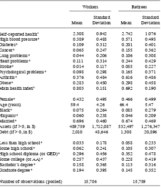
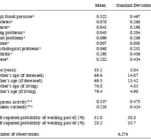
from retirement. After omitting observations with missing values for key variables, the fi nal sample size is 31,545 pooled observations for 6,276 distinct individuals. This provides an average longitudinal depth of fi ve time periods per individual, or about ten years. Table 1 contains summary statistics of key variables in the pooled sample, conditional on labor force status. Table 2 contains summary statistics for key initial period variables including those that form the instrument set.
C. Health Measurement
Various indexing techniques are common in health literature, including weighting, factor analysis, and item response theory methods.12 This paper adopts the fi rst option;
the primary health measure is derived from a straightforward weighting scheme. Ro-bustness checks in Section V compare various alternate weighting schemes. Although omitted from the text, item response health indices did not produce substantially dif-ferent results, either in their qualitative characteristics or their statistical signifi cance. In general, the main health index is a weighted sum of “objective” doctor- diagnosed health variables and “subjective” self- reported health status.
A health index reduces relevant health- related information to a scalar value that represents general health. In order to use regression analysis to explain variation in health changes, it is necessary to assume that health is a unidimensional trait (because it is the dependent variable). The index is built from ten categorical variables. One is an ordinal response “subjective” self- reported health variable,13 and the rest are
11. Section V includes a robustness check that alters the defi nition of retirement.
“objective” binary response doctor- diagnosed health conditions. They include heart problems (heart attack, coronary heart disease, angina, or congestive heart failure), high blood pressure or hypertension, stroke or transient ischemic attack, diabetes or high blood sugar, chronic lung disease (aside from asthma), arthritis or rheuma-tism, cancer (aside from benign skin cancer), psychological problems (emotional, Table 1
Summary Statistics: Workers and Retirees
Workers Retirees
Mean
Standard
Deviation Mean
Standard Deviation
Self- reported healtha 2.308 0.942 2.742 1.076
High blood pressure* 0.389 0.488 0.571 0.495
Diabetes* 0.109 0.312 0.201 0.401
Cancer* 0.065 0.247 0.155 0.362
Lung problems* 0.044 0.206 0.106 0.308
Heart problems* 0.111 0.314 0.244 0.429
Stroke* 0.014 0.117 0.055 0.227
Psychological problems* 0.098 0.298 0.165 0.371
Arthritis* 0.376 0.484 0.616 0.486
Obese* 0.283 0.450 0.298 0.458
Main health indexb 0.803 0.151 0.692 0.190
Female* 0.432 0.495 0.466 0.499
Age (years) 59.4 4.26 66.4 5.47
Black* 0.075 0.264 0.085 0.279
Hispanic* 0.060 0.238 0.046 0.209
Married* 0.696 0.460 0.674 0.469
Assets (if > 0, in $) 489,759 1,712,087 532,497 1,276,347
Debt (if > 0, in $) 2,010 48,646 1,308 20,896
Less than high school* 0.033 0.178 0.058 0.233
Some high school* 0.062 0.241 0.105 0.307
High school diploma (or GED)* 0.296 0.456 0.352 0.478
Some college (or AA)* 0.257 0.437 0.228 0.419
Bachelor’s degree* 0.158 0.365 0.113 0.316
Graduate degree* 0.194 0.395 0.145 0.352
Number of observations (pooled) 15,786 15,759
Notes: *Binary indicator; estimates refer to sample proportions rather than sample averages. a. 1 ~ Excellent health, 2 ~ very good, 3 ~ good, 4 ~ fair, 5 ~ poor.
nervous, or psychiatric problems), and obesity (indicated by a body- mass index14
greater than 30).15
Bound et al. (1999) provide the framework for the construction of the main health index. They performed an ordered probit regression of self- reported health on a set of objective health characteristics. They then formed predictions of self- reported health for each individual based on the probit results, and those predictions became the fi nal index. As all covariates were objective health characteristics, variation in the index was produced solely by individual differences in those objective health categories. Table 2
Summary Statistics: Initial Period Characteristics
Mean Standard Deviation
High blood pressure* 0.322 0.467
Diabetes* 0.078 0.268
Cancer* 0.041 0.198
Lung problems* 0.043 0.204
Heart problems* 0.090 0.286
Stroke* 0.007 0.085
Psychological problems* 0.068 0.251
Arthritis* 0.295 0.456
Obese* 0.252 0.434
Age (years) 55.1 3.04
Mother’s age (if deceased) 69.6 14.07
Father’s age (if deceased) 69.3 13.42
Mother’s age (if living) 76.8 4.83
Father’s age (if living) 79.4 4.98
Vigorous activity?a* 0.337 0.473
Smokes currently?b* 0.235 0.424
Self- reported probability of working past 62 (%) 51.0 38.8
Self- reported probability of working past 65 (%) 28.2 33.7
Number of observations 6,276
Notes: *Binary indicator; estimates refer to sample proportions rather than averages. a. Whether respondent engages in “vigorous physical activity” three or more times a week. b. Whether respondent is “a current smoker.”
14. Calculated by dividing an individual’s self- reported weight in kilograms by his or her self- reported height in meters squared.
Subjective self- reported health contributed only in the calculation of the probit
coef-fi cient estimates, thereby determining “weights” for each doctor- diagnosed condition. In the current study, the main model uses a modifi ed technique to produce variation from both objective health conditions and self- reported health. The index is con-structed as follows:
1. Estimate ten separate probit models, each one with a different health con-dition on the lefthand- side and the remaining nine health concon-ditions on the righthand- side. (Note that this set of 10 includes all objective conditions as well as self- reported health.)
2. For each probit model and for each observation, generate a prediction of the dependent variable.
3. For each probit model, normalize the predictions to lie between zero and one, where outcomes closer to one indicate better health.
4. For each observation, average across all ten predictions to calculate the obser-vation’s fi nal health index.
Such a procedure allows for an unprejudiced weighting scheme, as it is unclear how to otherwise integrate variation from both objective and subjective sources into the index. An alternate option would be to use a dependent variable that is not indicative of a dis-tinct health characteristic in the “weighting- choice” probit model. Section V contains a robustness check using a variable regarding health- related work limitations on the lefthand side, as well as a check using a pure form of the Bound et al. (1999) index.
In developing a health index, it is important to consider the usefulness of includ-ing both “subjective” and “objective” survey information. On the one hand, there is evidence that “objective” variables are not, in fact, free of biases. Baker, Stabile, and Deri (2004) matched health- related Canadian survey data with respondents’ offi cial health records, fi nding strong evidence of both false negatives and false positives in the self- reported, “objective” ailment reports. This casts doubt on the idea that there is a clear distinction between “objective” and “subjective” indicators and implies that measurement error may enter the discussion (Section IVD further develops this is-sue). On the other hand, there is a clear distinction between the two types of health information based on survey- question wording: “Subjective” self- reported health (on a discrete scale from one to fi ve) is very broad, while “objective” ailment queries are quite specifi c. Thus a natural concern is the extent to which including subjective indicators in the health index enhances its explanatory power: What, if anything, does subjective health add, after controlling for objective measures?16
Because a stated goal of this paper is to compute a health index that best represents “general health,” such an index must incorporate as much relevant health- related information as possible. Many researchers in the health- labor fi eld have estimated their results using objective and subjective health indicators separately, often fi nding differences that stem from the objective- subjective choice.17 Indeed, the
discrepan-cies themselves provide evidence that “subjective” measures contain something that
16. For instance, in implementing a version of the Bound et al. (1999) index, Coe and Zamarro (2011) refer to “multicollinearity problems that arise when including both objective and subjective measures of health as controls.”
objective measures do not. (The question of whether that something includes “good” health- related information or “bad” noise is left for Section IVD.) Others have em-ployed health indices that simultaneously incorporate subjective and objective in-formation.18 Since such an index is utilized extensively below, it is also valuable to
formulate a simple test to ensure that subjective indicators do indeed supplement the objective health information: Estimate a Bound et al. (1999)- style ordered probit with self- reported health regressed on the nine doctor- diagnosed ailment conditions, and then check various goodness- of- fi t criteria to ensure that the self- health grades are not “too strongly” predicted. For the main HRS sample, some corresponding fi t- metrics are McFadden’s pseudo R2 of 0.103, Cox & Snell’s pseudo R2 of 0.255, and an
ad-justed count R2 of 0.102, which captures the predictive power on top of the baseline
count R2 of 0.418 from the intercept- only model. Thus there is strong evidence that
doctor- diagnosed ailments provide some predictive power for self- reported health, but there is still a large component of those health scores that remains unexplained.
IV. Econometric Model
This section presents the theoretical foundation of the empirical work. The fi rst step is to investigate the baseline ordinary least squares (OLS) model and its limitations. The derivation of the corrected form of the model follows.
A. Baseline Model (OLS)
In the following model, t is the survey period, i is the individual, and Xit is a set of exogenous controls that include age, years of education, gender, race, marital status, log of value of assets, and log of value of debt.19RS
it (“short- term” retirement) is a
dummy variable indicating that individual i retired in period t (but not before). RLit
(“long- term” retirement) is equal to one only when i retired in period t – 1 or before. Thus the retirement effect has two components: RSit measures the short- term effect of recent retirement that occurred since the previous survey, and RLit gauges the cumula-tive effect of retirement spells that are at least one time period (or two years) long. Specifi cations that further discretize the cumulative effect require additional lags of re-tirement, constraining the sample signifi cantly.20∆H
it is the change in the health index.
A health change value less than zero corresponds to a decline in health. μit includes all unobserved factors that drive changes in health. The baseline specifi cation is:21
18. Lange and McKee (2011); McHorney and Cohen (2000); Madrian, Mitchell, and Soldo (2007); Ware et al. (1995).
19. Log of debt and log of assets are conditional on debt and assets being greater than zero, respectively. In other words, log of debt (or assets) is set equal to zero if the observation’s debt (or assets) level is less than one dollar.
20. In the case of a three- period discretization, a minimum of four observations would be required: four time periods permit three observed health changes, one for each of the necessary three observations of retirement status. Such a restriction would eliminate approximately one quarter of the sample.
(1) ∆Hit = βXit + θ1RSit + θ2RLit + μit
The dependent variable is health change instead of health level because postretirement health changes are not susceptible to the simultaneity problem (retirement- causing health declines are no longer an issue because retirement has already occurred). How-ever, retirement is still endogenous. RSit and RLit are correlated with μit because an individual’s retirement decision may depend on health- related events that are unob-served (to the econometrician), biasing coeffi cient estimates. Estimates of θ1 will be biased downward because retirement- causing health shocks between periods t and
t – 1 will be picked up by the RSit indicator. OLS estimates of θ2 may also suffer down-ward bias due to anticipated health declines that may be correlated with retirement.22
B. Corrected Model (IV)
An instrumental variables strategy aims to account for endogeneity in retirement. It is helpful to split the error term μit into three pieces. Let fi represent fi xed (by individual) unobserved heterogeneity correlated with health change, let ait include time- variant unobserved health effects that are anticipated by the individual, and let uit include all other (unanticipated) time- variant unobserved effects:
(2) μit = fi + ait + μit
ait may be correlated with retirement because it encompasses hidden health charac-teristics (in particular, health expectations) that are naturally tied to the retirement decision. For instance, a worker might hold private knowledge about a hereditary heart condition that compels him or her to retire before its actual onset. uit may be cor-related with retirement due to unanticipated between- period health shocks infl uenc-ing an individual’s retirement decision. Lastly, fi contains any possible time- invariant unobservables; retirement- related hidden anticipations could also lie in fi.
The instrument set is based on two key questions from the HRS questionnaire: “What do you think the chances are that you will be working full- time after you reach age 62?” (There is an analogous question for age 65.) Because the sample includes only individ-uals who entered the survey while employed, these inquiries provide valuable informa-tion about their retirement preferences and expectainforma-tions. Their responses are (by con-struction) uncorrelated with unanticipated retirement- causing health shocks uit, because they are taken from individuals’ initial observations, which preceded their retirement.
The retirement expectations instruments are likely correlated with ait, so the next step is to orthogonalize them to a set of proxies for ait. As with the instruments, the proxy variables are taken from each individual’s initial period of observation. They in-clude parents’ age Pi0, the respondent’s initial age AGEi0, original- period health level indicators HIi0, and original- period health behaviors HBi0.23 The IV strategy relies on
22. For instance, bias could be caused by diagnoses of ailments that are degenerative. Or, an individual may be aware of a predisposition for cancer and plan his or her retirement accordingly. Bias could also come through health events that occur very close to the survey date that impact labor supply choices.
23. In the regressions, Pi0 is split into four variables: mother’s age at death (or equal to zero if still living), mother’s current age if still living (or equal to zero if deceased), and likewise for the father’s status. HIi0
the assumption that the residuals from the following two regressions are orthogonal to ait:24
(3) Pr(Working past 62)i0 = ψ1Pi0 + γ1AGEi0 + δ1HIi0 + λ1HBi0 + ε1,i0
(4) Pr(Working past 65)i0 = ψ2Pi0 + γ2AGEi0 + δ2HIi0 + λ2HBi0 + ε2,i0
For this assumption to hold, the set of proxies must be correlated with the component of retirement expectations that is linked to future health change. In other words, the following must hold (where ε̂1,i0 and ε̂2,i0 are the residuals):
(5) corr({ε̂1,i0, ε̂2,i0}, ait) = 0
The next subsection discusses this assumption in more detail.
The last step in constructing the instrument set is to generate interactions of the residuals with binary indicators of whether the individual is under age 62 or is age 62–65 (to refl ect discontinuous retirement incentives at these ages due to Social Secu-rity and Medicare eligibility). Thus the instrument set is six- dimensional:
1. Under- 62 dummy 2. Age 62–65 dummy 3. ε̂1,i0
4. ε̂2,i0
5. ε̂1,i0 × Under- 62 dummy 6. ε̂2,i0 × Age 62–65 dummy
The interaction terms function as slope- differentials for the dummies, and the instru-ment set as a whole yields a strong fi rst- stage regression. It is overidentifi ed, which permits validity tests of the corrected model (results in Section V). The dummy variable interactions also ensure that the residual component is time variant, allow-ing fi xed effects specifi cations to be used to address potential endogeneity stemming from fi.
The fi nal model utilizes two stage least squares (2SLS) to estimate Equation 1, instrumenting endogenous variables RSit and RLit with the variables described above. 2SLS yields consistent estimates of the regression coeffi cients under the assumptions previously discussed and in the next subsection.
C. Instrument Validity
In order for estimates of θ1 and θ2 to be consistent, the standard IV assumptions must be satisfi ed. The fi rst- stage regressions imply that the instrument set strongly predicts retirement in each period.25 The crucial assumption is that the instruments must be
uncorrelated with μit, which can be decomposed into the three components seen in Equation 2. The instruments are orthogonal to uit by construction, and fi xed- effects can circumvent possible correlation with fi. However, the instruments must also be uncorrelated with ait. Recall that the instrument set has two components: residuals cal-culated from orthogonalization Equations 3 and 4 as well as age dummies. Exogeneity of the age dummies follows because individuals are not predisposed to have certain
health shocks at those ages versus any other similar age. They are linked to retirement because 62 and 65 are the entitlement ages for Social Security and Medicare ben-efi ts. Thus it remains only to argue that Equation 5 holds. The retirement expectations instruments—Pr(Working past 62)i0 and Pr(Working past 65)i0—contain two main pieces of information about an individual:
1. Information on retirement expectations 2. Information on retirement preferences
Individuals’ retirement preferences contain only exogenous variation that is correlated with their actual retirement. Individuals’ retirement expectations may be endogenous because they are tied to their health expectations (namely, both the instruments and
ait contain this information). The hypothesis is that individuals form their hidden (to the econometrician) retirement- related health expectations based on hereditary health trends (proxied by parents’ age) and past health history (proxied by initial- period health levels, behaviors, and age). Thus the “expectations component” is removed from the orthogonalized instruments ε̂1,i0 and ε̂2,i0, leaving only exogenous variation in retirement preferences. If the set of proxies omits crucial information that is correlated with ait, then estimates may be biased downward due to anticipated retirement- causing health shocks.26 In summary, instrument validity relies on the assumption that the
proxies are robust enough to predict anticipated effects. If this holds, 2SLS estimates of the regression parameters are consistent.
It is reasonable to suspect that parents’ age and initial health are inadequate proxies for the component of expected health that is contained in the retirement expectations variables. In this regard, it is helpful to estimate IV models using the “uncleaned” instruments, Pr(Working past 62)i0 and Pr(Working past 65)i0, in place of the “cleaned” residuals, ε̂1,i0 and ε̂2,i0, in the instrument set. The discussion below omits these estima-tion results for brevity, but it is important to note that they do not differ signifi cantly from the main results.27 “Uncleaned” instruments yield IV estimates of θ that are
slightly less statistically signifi cant, but corresponding Sargan- Hansen J- statistics are indistinguishable from those of the main model. This suggests that the proxies are not strong predictors of expected health, but at the same time, “improperly cleaned” expected health information does not seem to adversely affect instrument validity. Thus it may simply be that individuals are not able to effectively forecast their future retirement based on their expected health evolution.
D. Measurement Error
Measurement error can be an issue when working with health indices. If it is present, then true health, hit, is unobserved. In this case, the econometrician observes:
(6) Hit = hit + ηit
where ηit is measurement error. There are two notable potential sources of measure-ment error. First, the health index may not capture all information that describes one’s
26. One can imagine less plausible stories with opposite bias, such as an individual who anticipates a health increase and subsequently retires in order take advantage of his newfound health.
health. In an ideal setting, the data would contain a complete set of health- related information such as cholesterol levels, blood and liver tests, nutrition, cardiovascular status, and an extensive disease history. All missing information is contained in ηit. However, the information included in the health index should be more descriptive of general health than such missing characteristics. For example, an individual who has a resting heart rate of 65 beats per minute may be healthier than one with a heart rate of 85 (all else equal), but pulse rate is not as consequential as doctor- diagnosed hypertension. These types of omissions may yield only classical measurement error in the dependent variable, thus infl ating standard errors. Even if this source of measure-ment error is not purely classical, any potential correlations between the error term and explanatory variables should be negligible because the health index contains enough crucial health- related information. For instance, a worker is less likely to retire on account of minor dental problems than he or she is after experiencing a heart attack. In any case, these types of issues would be corrected via the IV specifi cation.
A second source of measurement error is known as “justifi cation bias,” which refers to retirees’ tendencies to exaggerate their poor health in order to provide so-cially acceptable justifi cation for their retirement. This phenomenon has been studied extensively by Bazzoli (1985), McGarry (2004), and others. Under such misreports, observed health would be understated for retirees, meaning that ηit may be correlated with RSit, RLit, or both. It is possible to show that the bias would work against the conclusion that retirement preserves health (thus making it harder to obtain signifi cant positive estimates of θ1 and θ2).28 If η
it represents justifi cation bias, it has the
follow-ing form:
Consider the following simplifi ed version of the structural Equation 1:
(8) ∆Hit = θ1RSit + θ2RLit + μit + ∆ηit
The size of the bias may be constant once an individual retires. In this case, ∆ηit is correlated with RSit but not with RLit. In either case, since the retirement expectations instrument is correlated with retirement, it is also correlated with ∆ηit. The next sec-tion shows that the fi nal estimate of RSit’s coeffi cient is zero and the fi nal estimate of RLit’s coeffi cient switches signs (negative to positive - going from OLS to 2SLS). Therefore, even if justifi cation bias does affect the corrected estimate of θ2, the 2SLS estimate serves as a lower bound for θ2 (and it is, at worst, masking a true positive value for θ1). In other words, justifi cation bias may act against the sign change, but the sign switches nevertheless. Note that the main source of justifi cation bias in the health index should be self- reported health. Given questionnaire wording, respondents are less likely to exaggerate their responses to the objective doctor- diagnosed conditions (but they still may, as mentioned above in reference to the work of Baker, Stabile, and
Deri 2004). As an additional test, the next section includes estimations of the model with a health index using only those objective conditions.
V. Main Results and Robustness Checks
This section reports the main empirical fi ndings and describes three robustness checks: a reestimation using a different defi nition of retirement, an exami-nation of the model’s predictions on various subsamples, and a comparison of the main estimates to those using alternate health indices which incorporate different weighting schemes or heath information.
A. Main Results
Table 3 displays four estimations of Equation 1:
1. Baseline model estimated by pooled OLS
2. Baseline model estimated via fi xed effects (FE) regression 3. Corrected model estimated via random effects (RE) regression 4. Corrected model estimated via fi xed effects regression
Insler
213
Dependent Variable: ∆Hit 1 2 3 4
Female 0.00124* 0.00137
(0.000732) (0.00108)
Age 0.0000228 –0.000856 –0.000508 –0.00478*
(0.00135) (0.00168) (0.00218) (0.00281)
Age2 –0.0000000 0.00000316 0.00000487 0.0000284
(0.0000105) (0.0000130) (0.0000168) 0.0000199)
Black 0.00345*** 0.00345**
(0.00115) (0.00158)
Hispanic 0.00402** 0.00394*
(0.00159) (0.00215)
Married –0.000152 –0.00712** –0.0000438 –0.00743**
(0.000908) (0.00313) (0.00122) (0.00314)
log(assets) 0.00118*** 0.000879 0.00116*** 0.000794
(0.000251) (0.000584) (0.000269) (0.000595)
log(debt) –0.000195 –0.000740 –0.000236 –0.000853
(0.000473) (0.000763) (0.000447) (0.000779)
Some high school 0.00565*** 0.00569**
(0.00206) (0.00260)
High school diploma 0.00684*** 0.00680***
(0.00184) (0.00232)
The Journal of Human Resources
Table 3 (continued)
Dependent Variable: ∆Hit 1 2 3 4
Some college 0.00584*** 0.00575**
(0.00192) (0.00243)
Bachelor’s degree 0.00893*** 0.00886***
(0.00203) (0.00268)
Graduate degree 0.00895*** 0.00893***
(0.00200) (0.00261)
Constant –0.0455 0.0109 –0.0316
(0.0431) (0.0537) (0.0699)
RLit: Long- term retirement –0.000148 0.00544*** –0.00223 0.0194*
(0.00102) (0.00207) (0.00446) (0.0101)
RSit: Short- term retirement –0.0137*** –0.00857*** –0.00827 0.0177
(0.00204) (0.00233) (0.0127) (0.0161)
Number of observations (pooled): 31,545 31,545 31,545 31,545
estimates change notably to 0.00544 and –0.00857, respectively. Following the work of Dave, Rashad, and Spasojevic (2008), short- term retirement is still negative since
fi xed effects do not cleanse estimates of between- period retirement- causing health shocks. The long- term retirement variable has switched sign but may still suffer from endogeneity bias, so the next step is to consider the IV specifi cations.
Table 4 contains the fi rst stage regression results for the corrected models (Models 3 and 4 in Table 3). The dependent variables are RSit and RLit, and the covariates include all exogenous regressors as well as the instruments excluded from the structural equa-tion. The instrumental variables are strong predictors of retirement. F- statistics from joint signifi cance tests of the instruments show that fi rst- stage regressions for long- term retirement are much stronger, although still at acceptable levels for short- term retirement in both RE and FE specifi cations. To interpret the instruments’ coeffi cient estimates, the residuals (ε̂1,i0 and ε̂2,i0) may be viewed as variables that are strongly and positively correlated with the expected retirement indicators, Pr(Working past 62)i0 and Pr(Working past 65)i0. For instance in Column 1, for an individual under 62, an additional percentage point in predicted probability of working past 62 corresponds to a –0.00229 + 0.00215 = –0.00014 (smaller) probability of being currently “long- term retired.” In Column 2, the same exercise yields a –0.000423 – 0.00144 ≈ –0.001 change in probability of being “short- term retired.”29 The coeffi cient interpretations
are qualitatively similar for the random effects model’s “working past 65” instruments, as well. In Columns 3 and 4, estimates for ε̂1,i0 and ε̂2,i0 are excluded due to the fi xed effects specifi cation, so it becomes more diffi cult to naturally interpret their interac-tions’ coeffi cients since the net effect depends on the unidentifi ed time- invariant fi xed effect. Thus the random effects fi rst stage regression is more easily interpretable and confi rms that the instruments are correlated to retirement in a logical manner.
Models 3 and 4 in Table 3 display the results from the IV specifi cations. Using random effects, the estimates of current period retirement and long- term retirement go to zero. A Sargan- Hansen test for Model 3 yields a J- statistic of 9.988 (p- value of 0.0406), rejecting that the instruments are exogenous. The IV fi xed effects specifi ca-tion, however, has a J- statistic of 0.523 (p- value of 0.7698), suggesting that one must account for time- invariant effects to attain instrument validity. Model 4 thus is the “fully corrected” model. The long- term retirement coeffi cient (θ̂2 = 0.0194) switches sign and can be interpreted as the local average treatment effect (LATE) of retirement on health change. Section VI discusses this in more detail. As one might expect, the “cumulative retirement” effect is much stronger than short- term retirement, whose coeffi cient estimate goes to zero in the fi nal model. Identifi able exogenous variables (age, assets, and marital status) do not substantially change across the four specifi ca-tions. The next three subsections test the robustness of these results.
B. Robustness Check: Alternate Defi nition of Retirement
One notable point of fl exibility in the econometric specifi cation is how to defi ne retire-ment. This is a central characteristic that is also related to the channels through which retirement may act upon health. For some individuals, retirement may simply refer to
The Journal of Human Resources
Table 4
First Stage IV Results
Dependent Variable RLit (RE) RSit (RE) RLit (FE) RSit (FE)
Female 0.0222*** –0.00782**
(0.00704) (0.00347)
Age 0.0119* 0.0817*** 0.0176** 0.0847***
(0.00641) (0.00598) (0.00805) (0.00621)
Age2 0.000176*** –0.000643*** 0.000138** –0.000669***
(0.0000481) (0.0000448) (0.0000613) (0.0000458)
Black –0.00515 0.00375
(0.0102) (0.00511)
Hispanic –0.0307** 0.00138
(0.0139) (0.00694)
Married 0.0132** –0.00891** 0.0208* 0.00227
(0.00638) (0.00393) (0.0124) (0.0107)
Log(assets) –0.00790*** 0.00157* –0.00592*** 0.00572***
(0.00123) (0.000868) (0.00174) (0.00169)
Log(debt) –0.0104*** 0.00368** –0.00888*** 0.00854***
(0.00173) (0.00144) (0.00219) (0.00226)
Some high school –0.0123 –0.00747
(0.0174) (0.00842)
High school diploma –0.0369** –0.00295
(0.0154) (0.00751)
Some college –0.0423*** –0.00255
Insler
217
Graduate degree –0.0408** –0.0137
(0.0170) (0.00840)
Under age 62 –0.231*** –0.0000872 –0.224*** –0.00387
(0.00814) (0.00802) (0.0107) (0.00952)
Age 62–65 –0.164*** 0.0753*** –0.160*** 0.0723***
(0.00609) (0.00608) (0.00799) (0.00796)
ˆ
ε1,i0 –0.00229*** 0.000423***
(0.000131) (0.0000678)
ˆ
ε2,i0 –0.00127*** 0.000165**
(0.000141) (0.0000714)
ˆ
ε1,i0 × Under–62 dummy 0.00215*** –0.00144*** 0.00227*** –0.00175***
(0.000107) (0.0000899) (0.000181) (0.000138)
ˆ
ε2,i0 × Age 62–65 dummy 0.000122 –0.00164*** 0.000196 –0.00168***
(0.000140) (0.000137) (0.000176) (0.000184)
Number of observations (pooled): 31,545 31,545 31,545 31,545
F- statistic: 2,016.92 596.34 173.49 85.47
their exit from the labor force. For others, it could refer to fewer hours on the same job or in the same career, or perhaps the opportunity to begin a new part- time career. The retirement indicator used in the main model was meant to accommodate this array of possibilities. However, if the fully corrected IV model truly captures a strong retire-ment effect on health, the effect should also be present under alternate defi nitions of retirement.
This test reestimates Models 1–4 using a new defi nition. In each wave, survey- takers respond to the question: “Are you currently working for pay?” This binary indica-tor forms a simple retirement dummy. Table 5 contains regression results. Estimates are qualitatively very similar those from the main model. Comparing baseline RE to corrected FE, the long- term retirement coeffi cient estimate goes from zero to a posi-tive value, while the short- term retirement estimate goes from a negaposi-tive value to zero. Using the alternate indicator, retirement estimates tend to be larger in absolute value. Various conjectures could explain the larger estimates: Complete nonwork may provide retirees with even more opportunity for healthy practices compared to partial retirees. Or, the set of “full retirees” may contain a larger proportion of individuals who were involuntarily forced out of the labor force due to injury or illness. In general, the main fi nding that retirement drives positive health changes appears intact.
C. Robustness Check: Estimation on Subsamples
The next robustness check reestimates the various models on two different sub-samples. Dave, Rashad, and Spasojevic (2008) suggested that healthier respondents and younger respondents should be less likely to experience sudden and severe ill-nesses leading to involuntary retirement. Under their hypothesis, retirement estimates in the baseline models should not be “as endogenous” as those from the main sample. Thus the relative change of baseline estimates to corrected ones should not be as large as in the main sample.
Table 6 contains retirement coeffi cient estimates from estimations restricted to these subgroups (the top portion of the table reproduces the main sample results for easy comparison). The younger subsample consists of only those survey respondents who entered the panel under age 58. The healthier subsample consists of only the individu-als who were in the top 75 percent of the initial- period health index distribution. Com-paring fi xed effects models (Model 2 to Model 4), the younger sample’s fi nal estimates are insignifi cant, but they increase (going from 0.00597 to 0.0146) by less than the main sample’s estimates (0.00544 to 0.0194). The same is true of the healthier sample, but statistical signifi cance is maintained in this case.30 These tests imply that the
cor-rective measures perform as intended on reasonable stratifi cations of the sample.
D. Robustness Check: Alternate Health Indices
The fi nal test performs estimations using two alternate health indices. The new health indices stem from similar calculations as the main health index detailed in
Insler
219
Dependent Variable: ∆Hit 1 2 3 4
Female 0.00122* 0.00140
(0.000734) (0.00109)
Age –0.000718 –0.000939 –0.00101 –0.00514*
(0.00131) (0.00165) (0.00218) (0.00273)
Age2 0.00000528 0.00000331 0.00000856 0.0000286
(0.0000102) (0.0000128) 0.0000169) (0.0000192)
Black 0.00387*** 0.00389**
(0.00116) (0.00159)
Hispanic 0.00329** 0.00320
(0.00159) (0.00215)
Married –0.000578 –0.00654** –0.000475 –0.00654**
(0.000915) (0.00312) (0.00122) (0.00315)
Log(assets) 0.00112*** 0.000608 0.00109*** 0.000544
(0.000248) (0.000585) (0.000269) (0.000602)
Log(debt) –0.000380 –0.00102 –0.000430 –0.00116
(0.000473) (0.000763) (0.000450) (0.000786)
Some high school 0.00453** 0.00446*
(0.00207) (0.00261)
High school diploma 0.00583*** 0.00562**
(0.00184) (0.00234)
The Journal of Human Resources
Table 5 (continued)
Dependent Variable: ∆Hit 1 2 3 4
Some college 0.00469** 0.00440*
(0.00191) (0.00246)
Bachelor’s degree 0.00720*** 0.00686**
(0.00202) (0.00272)
Graduate degree 0.00729*** 0.00697***
(0.00199) (0.00268)
Constant –0.0185 0.0180 –0.0123
(0.0420) (0.0525) (0.0693)
RLit: Long- term retirement 0.000917 0.00781*** –0.00243 0.0283**
(0.000991) (0.00211) (0.00503) (0.0133)
RSit: Short- term retirement –0.0164*** –0.0101*** –0.0132 0.0380
(0.00218) (0.00249) (0.0175) (0.0249)
Number of observations (pooled): 31,491 31,491 31,491 31,491
Insler
221
Dependent variable: ∆Hit 1 2 3 4
Main results (reproduced from Table 3)
RLit: Long- term retirement –0.000148 0.00544*** –0.00223 0.0194*
(0.00102) (0.00207) (0.00446) (0.0101)
RSit: Short- term retirement –0.0137*** –0.00857*** –0.00827 0.0177
(0.00204) (0.00233) (0.0127) (0.0161)
Number of observations (pooled): 31,545 31,545 31,545 31,545
Younger subsample (initially under age 58)
RLit: Long- term retirement –0.000382 0.00597*** –0.00404 0.0146
(0.00113) (0.00229) (0.00505) (0.0119)
RSit: Short- term retirement –0.0152*** –0.00927*** –0.00312 0.0201
(0.00224) (0.00253) (0.0150) (0.0179)
Number of observations (pooled): 25,848 25,848 25,848 25,848
Healthier subsample (initially top 75 percent of health distribution)
RLit: Long- term retirement –0.00148 0.00364* –0.00209 0.0169*
(0.00105) (0.00210) (0.00452) (0.0100)
RSit: Short- term retirement –0.0140*** –0.00909*** –0.00255 0.0209
(0.00212) (0.00239) (0.0130) (0.0163)
Number of observations (pooled): 28,889 28,889 28,889 28,889
Section III. The fi rst index is similar to that of Bound et al. (1999) and is calculated as follows:
1. Estimate an ordered probit model with a self- reported health on the side and the remaining nine “objective” doctor- diagnosed conditions on the righthand- side.
2. Generate predictions of the self- reported health observations from the probit estimation.
3. Normalize the predictions to lie between zero and one, where outcomes closer to one indicate better health.
The variation in the index comes only from individuals’ responses to the objective health questions (although it is scaled by their relation to self- reported health). Table 7 contains retirement estimates of the four econometric specifi cations using this index (it reproduces the main results in the top panel). Baseline estimates (Models 1 and 2) using the Bound et al. (1999) index are qualitatively similar to the estimate of the main model, although FE causes the coeffi cient estimate for RLit to go to zero. The fully corrected model yields statistically insignifi cant results that are negative.
Other studies have encountered this (lack of signifi cance) issue when using purely objective measures, including Neuman (2008) and Bound and Waidmann (2007). A possible explanation is due to a “role bias”: Retirees may feel healthier than they did while working because their role in retirement is less physically or mentally de-manding. In this situation, subjective self- reported health may be infl ated because retirees’ “perceived health” improves, even without any changes in “real health,” which would be refl ected in objective health indicators. This would bias estimates of retirement’s effect upwards in the main model, explaining why the Bound et al. (1999) (the ailment- condition- only) index does not capture an effect. An alternate explanation, as discussed in Section IIIC, is that objective measures simply do not possess enough information to capture retirement’s effect under the IV estimation strategy. There is strong evidence, from both related literature and simple empirical exercises described in Section IIIC, that subjective health variables enhance health measurement. Such evidence refutes the “role bias hypothesis” by indicating that it is the loss of information that causes the loss of signifi cance, not the loss of an upward bias.
Since it may be more appropriate to use health indices that employ both objective and subjective health characteristics, the main results should be robust to alternative indexing schemes using both types of information. The third panel of Table 7 presents reestimations of the four models using a jointly objective and subjective health index, again derived from the Bound et al. (1999) indexing technique, with two differences: The lefthand- side variable of the probit model is a binary indicator of whether “health limits [the respondent’s] ability to work” and the righthand- side variables now include self- reported health dummies in addition to the nine doctor- diagnosed conditions. Re-sults are qualitatively similar to the main reRe-sults with the exception that the short- term retirement estimate is now signifi cant at the 5 percent level. Estimates using this index tend to be larger in absolute value than the main estimates, but it is not safe to compare across the two models since they have different dependent variables.
Insler
223
Dependent variable: ∆Hit 1 2 3 4
Main results (reproduced from Table 3)
RLit: Long- term retirement –0.000148 0.00544*** –0.00223 0.0194*
(0.00102) (0.00207) (0.00446) (0.0101)
RSit: Short- term retirement –0.0137*** –0.00857*** –0.00827 0.0177
(0.00204) (0.00233) (0.0127) (0.0161)
Number of observations (pooled): 31,545 31,545 31,545 31,545
Bound et. al (1999) (self- reported health weighted) index
RLit: Long- term retirement –0.00395*** –0.00236 –0.00354 –0.00414
(0.000868) (0.00155) (0.00293) (0.00689)
RSit: Short- term retirement –0.0114*** –0.00863*** –0.00621 –0.00361
(0.00138) (0.00157) (0.00834) (0.0112)
Number of observations (pooled): 31,545 31,545 31,545 31,545
Health- limiting weighted index
RLit: Long- term retirement –0.000782 0.00905*** 0.00138 0.0399**
(0.00160) (0.00320) (0.00713) (0.0159)
RSit: Short- term retirement –0.0300*** –0.0207*** 0.00923 0.0598**
(0.00346) (0.00386) (0.0203) (0.0257)
Number of observations (pooled): 31,545 31,545 31,545 31,545
includes the more “broadly based” subjective self- reported health. This is an avenue for future research, as there are many possible methods for health measurement.
VI. Interpretation
This section explores the main fi ndings in more detail. The fi rst sub-section relates changes in the health index to specifi c ailment conditions in order to better interpret the magnitude of the retirement effect. The next subsection investigates adaptions of the main model in order to observe the direct association of retirement with two factors—smoking and exercise—that may drive its benefi cial infl uence on health. These analyses motivate some simple policy- related exercises at the end of the section, which demonstrate practical applications of the model.
A. Interpretation of Main Results
The previously provided interpretation for the corrected estimate of θ2 was that an av-erage length retirement spell (7.4 years, conditional on retirement having occurred two or more years before the latest survey) is associated with a health index that is 0.0194 points higher, holding all other observables fi xed. Following the work of Angrist, Im-bens, and Rubin (1996), this coeffi cient has an additional causal interpretation as the local average treatment effect (LATE) of retirement on health change. The calculated effect is attributable specifi cally to subpopulations who are affected by changes in the instruments. In other words, θ2 represents the average effect of retirement on health changes for the subpopulation who responds to retirement preferences and age- based (62 and 65) incentives. An important caveat is that this empirical approach does not reveal anything about the retirement effect amongst the set of individuals who would always retire at a certain point regardless of those characteristics. Thus the LATE does not apply to individuals who experience involuntary retirement due to illness or injury.
A regression decomposition of the health index provides a framework for more concrete interpretation of the LATE. Table 8 presents a simple OLS regression of the health index on the nine ailments as well as self- reported health dummies. (It also presents regression results for the health indices used in the robustness checks.) Hold-ing self- reported health constant, high blood pressure, diabetes, and heart problems carry the highest weight in the main health index. Cancer possesses a surprisingly low weight, perhaps implying that its effect is “washed out” by the self- reported health covariates. Applied to Table 8, the main retirement estimate θ̂2 = 0.0194 indicates that the LATE of retirement on health change (over the average observed length of a long- term retirement spell, which is 7.4 years) is approximately equivalent to prevention of “one- quarter” of a doctor- diagnosed condition such as arthritis, or smaller fractions of more severe ailments. Alternatively, it implies that a 7.4 year long retirement spell should prevent arthritis for one in four individuals.