Family Labor Supply
Paul J. Devereux
A B S T R A C T
The large changes in relative wages that occurred during the 1980s provide fertile ground for studying the behavioral responses of married couples to the wage changes of husbands and wives. I find estimates of own-wage and cross-wage elasticities for men that are very small. The own-wage elasticity for women is positive and the cross-wage elasticity for women suggests a strong negative response of female labor supply to changes in their hus-band’s wages. Family labor supply behavior determines how changes in individual wage rates translate into family earnings changes. The responses of women to changes in their husband’s wages attenuated somewhat the increases in individual wage inequality at the family level: The results sug-gest that the earnings of the wives of low-income men would actually have fallen over the decade if women’s labor supply did not respond to changes in their husbands’ wages. However, assortative mating implies that wage changes of husbands and wives are correlated and so family earnings inequality still grew during the decade of the 1980s.
I. Introduction
In the absence of behavioral responses, changes in individual wages will mechanically result in changes in family earnings inequality. However, both hus-bands and wives can adjust their labor supply in response to changes in their own wage and in their spouse’s wage. The size and direction of these responses determine the actual impact of changing individual level wage inequality to the family. Ultimately, understanding what happens at the family level is important since so much of social policy is aimed at this level. The 1980s were a decade of enormous change
Paul J. Devereux is a professor of economics at the University of California, Los Angeles. He thanks Dan Ackerberg, Janet Currie, Eric French, Phillip Leslie, Kanika Kapur, and participants at the Summer Meetings of the Econometric Society and the Rand UCLA Labor and Population Seminar for helpful comments. The data used in this article can be obtained beginning January 2005 through December 2008 from Paul Devereux, UCLA, email: devereux@econ.ucla.edu.
[Submitted November 2001; accepted May 2003]
in relative wages affecting both men and women. During this period, the college wage premium increased dramatically and real wages of less-educated men fell. In this paper, I study the behavioral responses of married couples to relative wage changes since 1979 and evaluate the role of these behavioral responses in mediating the result-ant changes in family earnings inequality.
Because female labor supply is more responsive than male labor supply, compen-satory labor supply behavior may be particularly important for wives responding to wage changes of their husbands. However, evidence from recent decades has cast some doubt on the importance of this response. Taking a synthetic cohort approach using United Kingdom data, Blundell, Duncan, and Meghir (1998) find small and sta-tistically insignificant income effects. They identify labor supply elasticities using changes in relative wages and income across groups of women defined by education and birth cohort. Thus, their finding implies that women whose husband’s income has fallen have not responded by increasing hours of work.
Juhn and Murphy (1997), among others, have shown that labor supply in the United States during the 1980s increased more for the wives of high-wage men than for the wives of low-wage men. Since the wages of low-wage men have fallen relative to the wages of high-wage men, this suggests that there is no strong relationship between changes in male wages and female participation. However, this conclusion ignores assortative mating—high-wage men are more likely to be married to high-wage women and so wives of men who experience positive shocks to their wages and labor supply are likely to experience the same positive shocks. Such assortative mating makes it difficult to test whether women have adjusted their labor supply in reaction to changes in husband’s wages. To examine labor supply behavior in the context of sizeable changes in relative wages of both men and women, it is necessary to estimate family labor supply functions that allow for changes in the relative wages of both men and women.
In this paper, I use repeated cross-sections from the 1980 and 1990 census to esti-mate models of family labor supply. I exploit the major changes in relative wages of both husbands and wives during this time period to identify the labor supply parame-ters of interest. In the estimation, I treat national and regional changes in relative wages as exogenous variation that can be used to identify labor supply responses. If labor is partially immobile across regions, relative wage changes will differ by region. It is well known that there are substantial differences across Census regions in the level and trend of measures of wage inequality (see, for example, Karoly and Klerman 1994) and across metropolitan areas (Borjas and Ramey 1995; Montgomery 1992). The approach I take is to use a grouping estimator to see how this cross-region varia-tion in relative wage changes across husbands and wives with different characteristics corresponds to the cross-region variation in relative labor supply changes.
men, in the absence of such behavior, the earnings of wives of low-wage men would not have increased at all.
II. Literature Review
Blundell and MaCurdy (1999) provide a summary of empirical work on family labor supply. There is a large cross-sectional literature that tends to treat wages as exogenous (Ransom 1987) or to use age or education as instruments for wages (Kooreman and Kapteyn 1986). Juhn and Murphy (1997) estimate cross-sectional labor supply equations and instrument individual wages with an indicator of the wage decile they are in. They find small wage and income effects for married women.
Pencavel (1998) provides a thorough study of the correlations between wages and hours worked by women between 1975 and 1994. He uses education, cohort, and trade variables, and interactions of these variables as instruments for the wages of wives and husbands. Thus, the identification strategy uses a mixture of cross-sectional sources (education and cohort) and time-varying elements (trade variables). He does not report a first stage regression so the extent to which time-varying variables play a role in the identification is unclear.
Cross-sectional strategies require strong assumptions to consistently estimate labor supply parameters. If taste for work is related to wages or to education, then cross-sectional estimation provides inconsistent estimates of own-wage elasticities. Obtaining consistent estimates is likely to be particularly difficult in models of fam-ily labor supply because assortative mating implies that unobservable characteristics of both spouses are likely to be correlated and also be related to the wages of each spouse.
Lundberg (1988) uses longitudinal data from the Panel Study of Income Dynamics (PSID) and takes a fixed effect simultaneous equation approach to the labor supply of husbands and wives. She finds evidence of compensatory behavior for families with young children but not for other families. A potential problem with this approach is that changes in wages are not random and may be related to fundamental changes to individual skills or attitudes. In contrast, my approach uses wage changes of the age-education group that are assumed to result from changes in the returns to skills in the economy, and hence are unrelated to tastes for work of husbands and wives.
cor-rect for small sample bias in different ways. Third, unlike BDM, I use variation across groups defined both by the type of husband and the type of wife and so I exploit vari-ation that arises because conditional on characteristics of the wife, there are pre-dictable differences in wage growth of husbands that are explained by husband characteristics such as age and education. This addresses the possibility that declin-ing wages of men occurrdeclin-ing alongside increasdeclin-ing hours of women may be purely a demand-side phenomenon (as suggested by Juhn and Kim 1999) rather than resulting from compensatory labor supply behavior. Fourth, I use regional variation in relative wage changes and labor supply behavior to relax the assumption that any changes in unobserved factors over time are the same for all education and age groups.
III. Data
To analyze wage and labor supply outcomes at the regional level for detailed demographic groups, I use data from the Public Use Micro Samples (PUMS) of the Census of Population in 1980 and 1990.1I use the 5 percent samples in each of these years. Such detailed analysis would not be possible using alternative sources of data such as the Current Population Survey (CPS) because they do not have nearly as many observations.
I restrict the sample to individuals who are aged between 21 and 60. Persons in school or the military during the survey week are omitted as are persons who are liv-ing in group quarters. I also exclude all cases where the husband or wife has self-employment income. The wage measure used is average hourly earnings where earnings include wage and salary earnings only. Earnings are topcoded at $75,000 in 1980 and $140,000 in 1990. Fewer than 1 percent of observations are topcoded in 1980 and the same is true in 1990. I replace the topcoded value by the topcode times 1.33 in both years. I deflate earnings using the personal consumption expenditures deflator.2I omit couples in which the husband does not work at all in the previous cal-endar year. With the exception of older men, participation rates are very high for mar-ried men in 1980 and 1990 so this is not a huge restriction. Both participating and nonparticipating women are included in the sample. I discuss the selection issues aris-ing from nonparticipation in the next section.
The labor supply measures refer to the hours worked in the previous calendar year and the wage measure is the log of average hourly earnings in the previous calendar year. I include three labor supply measures. The first, Hours, is annual hours worked. The second, Full Time⎪Full Year(FTFY), is an indicator for individuals who worked at least 50 weeks and usually worked 35 or more hours per week. The third, Annual
1. I do not use the 1970 census because there is no information on usual weekly hours last year, and weeks worked is bracketed. Hence, some strong assumptions are required to calculate average hourly earnings and hours worked. See Pencavel (1997) for more detail on the drawbacks of making these assumptions. Furthermore, the available sample sizes are inadequate for the approach taken in this paper.
Participation, is an indicator for people who worked for even one hour in the year. Like Juhn (1992), Welch (1997), and Devereux (2003), I make no distinction between periods of nonemployment that are classified as unemployment and periods spent out of the labor force.
IV. A Specification for Family Labor Supply
I assume a simple linear model of labor supply behavior of husbands and wives. The wife’s labor supply is given by:
( )1 hf=α0+α1wf+α2wm+α3Y+α4Z+vf
where hfis the log of annual hours worked by the wife, wfis the log of her hourly wage rate, wmis the log of the husband’s hourly wage rate, Yis the nonlabor income of the family, Zis a vector of other controls, and vfis a stochastic error. The labor sup-ply function for husbands is as follows:
( )2 hm=β0+β1wf+β2wm+β3Y+β4Z+vm
These labor supply functions are appropriate for the current problem because the identification strategy is to use changes in relative wages to identify the labor supply parameters. Thus, this parameterization of labor supply as a function of the wages of husband and wife enables the identifying assumptions to be used in a simple and clear fashion.
The emphasis in this paper is on the effects of changes in relative wages on hours worked and how these feed through into changes in the distribution of family earn-ings. Given the focus on the distribution of earnings across families, I interpret coef-ficients in terms of the standard unitary model of family labor supply. It is worth noting that nonunitary models of family labor supply would imply different interpre-tations of the estimated coefficients. For example, in collectivist models of labor sup-ply, changes in wages influence hours in part through their effect on the bargaining power of individual spouses and hence on the sharing rule. Blundell and MaCurdy (1999) provide a discussion of the characteristics of unitary and collectivist models of family labor supply, Chiappori (1988, 1992) develops the labor supply model from a collective perspective, and Blundell et al. (2001) show how collectivist models can be identified and estimated when not all individuals participate. These models are par-ticularly useful for evaluating changes in the intra-household distribution of welfare. The wage and other income variables in Equations 1 and 2 must be considered to be endogenous because of measurement error and unobserved characteristics that are correlated with wages, nonlabor income, and hours worked. Thus, I take an instru-mental variables approach to the estimation of these equations. Because I am inter-ested in exploiting changes in relative wages across groups to identify the parameters, the instruments used are group indicators. This instrumental variables approach can be shown to be exactly equivalent to grouping the data and regressing the group mean of hours on the group means of the right hand side variables using weighted least squares (Angrist 1991).
variables for each group are observed in 1980 and 1990. These groups are the inter-actions of husband type with wife type and with region. In all analyses, the group means are weighted by the number of underlying observations in each group. The details about how the groups are defined are below in Section VI.
Nonparticipation
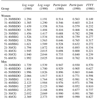
The sample is restricted to married couples in which the man participated at some point in the calendar year but includes both participating and nonparticipating wives. Of the 1,266,752 wives in 1980, 62 percent participate; 74 percent of the 1,271,815 wives in 1990 participate. In this paper, both hours and participation models are esti-mated for wives. The usual selection problem arises with hours only being positive for participating women and wages being unobserved for nonparticipators. The problem is ameliorated somewhat because, as we shall see, the models are estimated in differ-ences so it is only changes in participation rates that cause a selection problem. However, there are sizeable increases in female participation over this period (see Table 1), so selection cannot be ignored.3In this section, I discuss the approaches taken to the selection problem when estimating Equation 1; in Section VII, I discuss wage imputation in the context of estimating participation equations.
In terms of the grouping estimation strategy, selection bias arises in the hours equa-tion due to changes in the composiequa-tion of working individuals that are not fully accounted for by the group and time effects used as controls. These biases will arise, for example, if an increase in the wage for a certain group leads to the entry into the labor market of individuals who work hours that are below average for the group. This would tend to bias the own-wage elasticity toward zero. Also if the fall in wages of low-skill men leads to entry of their wives into the labor market at hours below aver-age for women like them, this would tend to bias the cross-waver-age elasticity toward zero. Theory can provide some guidance about the selection problem. If individuals dif-fer in taste for work, then individuals who are less likely to participate are also less likely to work long hours if they participate. Thus, we would expect groups who increase participation rates to add individuals to the workforce who have low taste for work and tend to work short hours. However, in the absence of further assumptions, theory provides no solution to the selection problems.
I take two approaches to the selection issue. The first approach (Correction 1) is to make structural assumptions about the error term distributions and do a selection cor-rection in the spirit of Heckman (1979) and Gronau (1974). I add as an extra regres-sor in the hours equation the inverse mills ratio evaluated at Φ-1(L
gt), where Φ-1is the inverse of the normal distribution and Lgtis the proportion of families in group g in which the wife participates in period t(see Blundell, Duncan, and Meghir 1998). This mills ratio term is added as an extra regressor in Equation 1 and the parameter δis estimated.4
3. The participation rates for married men have not changed very much (although there is some evidence of a decline in the participation rates of high school dropouts).
The second approach (Correction 2) is to use the insight from theory than marginal participators are likely to work lower hours than other observationally equivalent individuals. Since theory cannot inform about how big the differences should be, I take the extreme approach of assuming that new participators come from the bottom tail of the hours distribution. The approach I take is to artificially truncate the sample so that the proportion of women in a group who work is maintained constant between 1980 and 1990. If a higher proportion work in 1990, individuals with the lowest hours in 1990 are removed until the proportions working are the same in 1980 and 1990. Analogously, if a higher proportion works in 1980 than 1990, individuals with the lowest hours in 1980 are removed so that the proportions remain the same. This approach is valid if the marginal participators in each group are from the left tail of
Table 1
Participation Behavior
Log wage Log wage Participate Participate FTFY FTFY
Group (1980) (1990) (1980) (1990) (1980) (1990)
Women
21-30/HSDO 1.294 1.191 0.514 0.563 0.149 0.190
31-40/HSDO 1.385 1.290 0.546 0.603 0.214 0.263
41-50/HSDO 1.439 1.358 0.516 0.579 0.232 0.283
51-60/HSDO 1.503 1.404 0.416 0.468 0.196 0.226
21-30/HSG 1.456 1.417 0.688 0.782 0.298 0.388
31-40/HSG 1.526 1.534 0.638 0.759 0.277 0.391
41-50/HSG 1.556 1.563 0.646 0.765 0.317 0.429
51-60/HSG 1.621 1.589 0.528 0.632 0.272 0.341
21-30/CG 1.794 1.872 0.834 0.893 0.334 0.495
31-40/CG 1.945 2.015 0.698 0.800 0.221 0.365
41-50/CG 1.940 2.044 0.733 0.840 0.239 0.371
51-60/CG 1.992 2.025 0.641 0.762 0.224 0.312
Men
21-30/HSDO 1.729 1.539 0.947 0.930 0.570 0.574
31-40/HSDO 1.890 1.700 0.929 0.905 0.627 0.595
41-50/HSDO 1.996 1.826 0.896 0.863 0.646 0.601
51-60/HSDO 2.066 1.917 0.813 0.771 0.598 0.540
21-30/HSG 1.911 1.764 0.982 0.981 0.736 0.766
31-40/HSG 2.123 1.984 0.976 0.971 0.798 0.791
41-50/HSG 2.207 2.123 0.960 0.952 0.810 0.793
51-60/HSG 2.252 2.168 0.894 0.877 0.737 0.701
21-30/CG 2.032 2.069 0.990 0.991 0.780 0.825
31-40/CG 2.369 2.373 0.989 0.990 0.827 0.857
41-50/CG 2.561 2.555 0.981 0.981 0.821 0.826
51-60/CG 2.598 2.604 0.940 0.933 0.777 0.737
the hours distribution of the group. Although this assumption is obviously an extreme one, the results should provide insight as to the possible impact of selection bias.
V. Identifying Assumptions
To fix ideas, consider the labor supply equation for wives after the data have been grouped: to wife type, and rrefers to region. So, for example, wijrtf is the average log wage at time tof a woman of type jmarried to a man of type iin region r. Types are defined by age and by education level.
I treat the group indicators (υijrf) as fixed effects. This feature distinguishes the framework from standard cross-sectional approaches in which education and/or age are excluded and used to instrument wages. Instead, I exploit changes in relative wages to estimate labor supply elasticities. The group dummies capture permanent differences in labor supply behavior between couples of different types. Some of this permanent variation reflects labor supply responses to permanent differences in wages but some will also reflect permanent differences in unobservables such as motivation that are correlated with both spouse’s wages.5I include couple dummies rather than individual dummies because assortative mating is likely to occur on the basis of unob-servables as well as obunob-servables. For example, a college graduate married to a high school dropout is likely to be different from a college graduate married to another col-lege graduate.
Because there are only two time periods, the estimation is carried out in differences. By differencing, one washes out the group fixed effects.
Taking differences, one arrives at Equation 5.
( )5 ijr
In all specifications, I treat the region-specific error component (∆ηrf) as a fixed effect and so there are region indicator variables in all specifications. Thus, I control
for region-specific factors such as local business cycles that may influence labor sup-ply. I estimate two specifications to reflect differing assumptions about the error com-ponent ∆µijf.
The first assumption is that ∆µijfis a random error component that is uncorrelated with each of the explanatory variables. Formally, E(∆µijf, ∆w
∆ =0. This implies that differences in female labor supply across groups, condi-tional on observable variables, remain constant over time. The identification comes from differences across groups in the rate of wage growth of husbands and wives between 1980 and 1990.
One might worry that in the estimator we are comparing hours changes in groups that are quite different (for example, men with college degrees to men without high school diplomas) and these groups may be subject to rather different unobserved shocks. If there is regional variation in changes in relative wages of men and women, one can exploit this variation to identify α1and α2by comparing the hours changes of couples with exactly the same education and age characteristics but different levels of wage growth because they live in different regions.
There are reasons to believe that the assumption that changes in unobservables affecting tastes for work are equal for all groups may be violated in the 1980 and 1990 census data. One issue is simply one of measurement: The questions and coding cat-egories for the education variables in the 1990 census differ from the corresponding ones in the 1980 census. While I try to make these variables consistent across the two years, there may still be changes in the composition of the groups between 1980 and 1990.6A second issue is the problem of identifying cohort, age, and time effects in repeated cross-sectional data. By grouping by age, I compare groups of similar ages in 1980 and 1990. This implies that the groups come from different cohorts and these cohorts may systematically differ in terms of tastes for work.
More generally, changes in societal norms and government policies on crime, drug use, consumerism, and other factors such as immigration may have had divergent influences on either the composition or the behavior of different groups. The problems may be especially large for wives since there have been rapid increases in labor mar-ket experience for women and a commensurate growing attachment to the labor market. These effects are likely to be greater for higher-skilled women and hence vio-late the assumption that changes in unobservables affecting tastes for work are equal for all groups.
Thus, in the preferred specifications, I allow for a correlation between ∆µijfand the
explanatory variables by including indicators for husband type and wife type in the differenced regression. Specifically, I allow changes in labor supply to depend on indicator variables that are formed by the interaction of the education categories (col-lege graduate, high school diploma, high school dropout), and age categories. Assortative mating implies that changes in unobservables are likely to be correlated
for husbands and wives. Therefore, I also include the equivalent controls for the type of the spouse.7
VI. Implementation of the Estimators
The large census sample sizes imply that detailed groups are feasible. The groups I use exploit changes in relative wages across regions and over time. I group the data based on education, age, and region. There are 1,296 groups defined by the inter-action of 12 husband types, 12 wife types, and 9 census regions. The 12 husband and wife types are defined by the interaction of three education categories (college graduate, high school diploma, high school dropout) and four age categories (21–30 years, 31–40 years, 41–50 years, and 51–60 years). I exclude persons who are less than 21 or more than 60. The choice of these 1,296 groups represents a tradeoff between detail and cell size.8
In practice the sample size of some of the groups is rather small—I use any group with five or more observations (on average, there are 843 observations per group in the hours equations, and 1,175 observations per group in the participation equations). When groups have small sample sizes, weighted least squares (WLS) estimates from regressions of the group means may suffer from small sample biases. As mentioned earlier, WLS on group means is equivalent to doing 2SLS with the individual-level data using group dummies as instruments. Correspondingly, this small sample bias is exactly equivalent to the well-known bias of 2SLS in finite samples (for example, see Bound, Jaeger, and Baker 1995). To deal with this bias issue, I implement an errors-in-variables estimator (UEVE) that is approximately unbiased in finite samples. This estimator is closely related to several bias-corrected instrumental variables estimators including Nagar’s estimator (Nagar 1959) and the Jackknife Instrumental Variables Estimator (see Devereux 2003 for a derivation of these relationships). The details about the implementation of this estimator are in Appendix A1.
An alternative approach to dealing with bias caused by small group sizes is to increase the number of observations per group by reducing the number of groups. Thus, I also implement an instrumental variables estimator where the instruments for ∆x-are interac-tions of region with husband type and interacinterac-tions of region with wife type.9Each obser-vation is weighted by the average number of obserobser-vations in the group in the two years. I refer to this estimator as the grouped two stage least squares estimator (G2SLS).
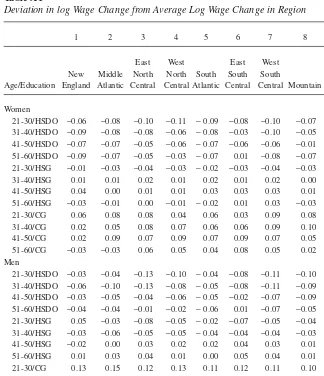
Table A1 provides some information about how wage changes differed among groups and between regions.10The numbers in the table are the deviation of the log
7. An alternative is to add controls for the 144 husband type*wifetype dichotomous variables. The results are almost identical when I do this. I choose the more parsimonious specification to save degrees of freedom. 8. I experimented with defining groups by race. Because relative wages have changed differentially for whites and nonwhites, I estimated separate regressions for each group. I found effects for white families that are similar to the results for all families. The estimates for nonwhite families were very noisy but the param-eter values suggested lesser behavioral response by wives both to changes in their own wages and changes in their husbands’ wages.
9. The cell sizes in the husband groups and the wife groups are large: On average, there are more than 8,000 observations in the wife type by region cells and husband type by region cells. Thus, any small sample biases are likely to be small with this estimation strategy.
wage change from the average log wage change in the region. One very clear effect is that educated groups had much larger wage increases than less educated groups (the numbers tend to become more positive as one moves down a column). The changes in relative wages are not uniform across region. For example, in the Pacific Division, male high school dropouts aged between 31 and 50 experienced relative wage cuts of about 15 percent, in the South Atlantic group the relative wage cut for this group was only 5 percent. The groups explain about 87 percent of the total variance in Table A1 for men, and 88 percent for women. The estimator exploits all the variation in Table A1 to estimate wage elasticities. However, the specifications that control for group indicators in the differenced regressions make use of the approximately 12 percent of the variation that is not explained by group effects.
A. Hours Elasticities for Wives
The estimates from the log hours equations of wives are in Table 2. In the first panel of Table 2, there is no correction for selection. Columns 1–3 contain the estimates without controls for husband and wife type, Columns 4–6 add controls for husband type and wife type in the differenced regression. I report results for all three estima-tors: These are weighted least squares (WLS), grouped two stage least squares (G2SLS), and the unbiased errors in variables estimator (UEVE).
First, consider how the elasticities differ across estimators. The WLS estimates of both the own-wage and cross-wage elasticities are smaller in absolute terms than the elasticities produced by the other estimators. A plausible explanation for this pattern is that measurement error in the sample means biases the estimated coefficients toward zero. It is worth noting that the WLS estimates are biased despite there being an average of 843 observations per group. Thus, in this application, both having the large sample sizes afforded by the Census and using estimators that correct for small sample bias are necessary in order to accurately estimate the behavioral responses. I will concentrate on the G2SLS estimates in the subsequent exposition. These gener-ally lie between the WLS and UEVE estimates both in terms of coefficient values and standard errors.
Next, consider the own-wage and cross-wage elasticities. In the specification in Column 2, the own-wage elasticity for women is 1.2. This elasticity is at the high end of estimates in the literature and suggests a very strong response of female labor sup-ply to increasing female wages.11As discussed elsewhere, it is likely that there have been shifts in female labor supply over time that make these estimates invalid. The estimates in Column 5 are robust to labor supply shifts that differ across wife types provided that they do not also differ across region. The own-wage elasticity from this specification is much smaller in magnitude and is approximately 0.2 (the implied compensated wage elasticity is approximately 0.75).12This smaller own-wage elas-ticity is similar to many of the recent estimates for women.
11. Hyslop (2001) and Pencavel (1998) find a compensated own wage elasticity for married women of about 0.4, both Ransom (1987) and Hausman and Ruud (1984) find elasticities of about 0.75. The compensated wage elasticity implied by my estimates of the uncompensated own wage elasticity and cross-wage elastic-ity is 1.75.
The cross-wage elasticity for women is very similar across specifications and is about −0.4. This suggests that a 10 percent fall in husband’s wage leads to a 4 percent increase in wife’s hours.13As such, this represents a sizable behavioral response by women to changes in their husband’s wage. The robustness of this estimate across the specifications in Columns 2 and 5 is reassuring and provides confidence in the simu-lations that are included later in the paper.14
Table 2
Estimates from Differenced Labor Supply Functions (Women)
WLS G2SLS UEVE WLS G2SLS UEVE
(1) (2) (3) (4) (5) (6)
Dependent Variable: Log(Annual Hours)
Log(wife’s wage) 0.713 1.193 1.242 0.002 0.174 0.381
(0.060) (0.073) (0.110) (0.055) (0.111) (0.292) Log(husband’s −0.128 −0.415 −0.447 −0.232 −0.385 −0.473
wage) (0.049) (0.058) (0.088) (0.045) (0.071) (0.129)
Nonlabor income −0.115 −0.081 −0.118 −0.109 −0.127 −0.421 *10,000 (0.086) (0.115) (0.139) (0.081) (0.168) (0.477)
Husband and wife No No No Yes Yes Yes
indicators
Dependent Variable: Log(Annual Hours): Corrections for Nonparticipation
Correction 1 Correction 2
Log(wife’s wage) 0.001 0.133 0.347 0.002 0.172 0.256
(0.055) (0.108) (0.285) (0.055) (0.111) (0.204) Log(husband’s −0.218 −0.342 −0.439 −0.236 −0.384 −0.456
wage) (0.045) (0.070) (0.130) (0.045) (0.071) (0.108)
Nonlabor income −0.087 0.002 −0.331 −0.106 −0.120 −0.409 *10,000 (0.082) (0.165) (0.467) (0.082) (0.168) (0.397)
Husband and wife Yes Yes Yes Yes Yes Yes
indicators
Standard errors are calculated using Huber-White covariance matrix. All specifications estimated in dif-ferences. Region indicators are included in all regressions. See text for details about corrections for nonparticipation.
bargaining position inside the household. Thus, hours respond both to the changes in the budget constraint resulting from the wage changes and also to the resultant changes in the weights placed on each individuals utility function within the household.
In the specifications with controls for husband and wife indicators, the own and cross-wage elasticities are generally similar in magnitude. This suggests that it may be the difference in the log wages that matters rather than the absolute level of the wages. However, tests for the linear restriction that wfand wh can be replaced by (wf−wh) generally reject the restriction. For example, for the estimates in Table 2, Column 5, the hypothesis is rejected using a conventional test for linear restrictions with a chi-square value of 21.
The second panel in Table 2 contains results where the two methods to deal with selection discussed in Section IV are implemented. Results are reported only for the specification with controls for husband and wife indicators. Reassuringly, the results with the Heckman-type correction, and the truncation correction are very similar to each other and to the uncorrected results. This suggests that the estimated elasticities are not suffering from severe selection biases.15
Nonlabor income is generally found to have a negative (but rarely statistically sig-nificant) effect on hours.16 Given the possible endogeneity of nonlabor income, it would be unwise to interpret this correlation as a causal effect. Excluding nonlabor income from the specification has little impact on the estimated wage elasticities.17
In unreported results, I have carried out the estimation using data grouped at the national level. At this level, there are 144 groups representing 12 husband types and 12 wife types. I find an own-wage elasticity for women of 1.25 (0.10) and a cross-wage elasticity of −0.44 (0.08). These are unsurprisingly similar to the results in Table 2 without the controls for husband and wife types. The similarity suggests that migra-tion across regions does not appreciably bias the estimates. Also, the estimates in Table 2 are robust to excluding nonnatives from the sample.
B. Hours Elasticities for Husbands
The hours elasticities for men are in Table 3. For men the estimates are quite similar across estimators and so I will concentrate on the G2SLS estimates. The own-wage elasticity is found to be very small and statistically insignificant in both specifications. These small elasticities are typical of male wage elasticities in the literature and sug-gest that married men do not adjust hours in line with small changes in wages.18The estimates for the cross-wage elasticity for men are positive for both specifications but are very small and statistically insignificant in Columns 4–6 of Table 3. This approx-imately zero cross-wage elasticity is certainly more plausible than the positive
wife’s wage, the less responsive her hours are to her husband’s wage. The fact that the wife’s hours are par-ticularly high when both she and her husband have high wages is consistent with leisure complementarities within the family.
15. When the wage elasticities are allowed to differ for families with and without children aged younger than 18, I find statistically insignificant differences in the wage elasticities for these two groups.
16. Nonlabor income is composed of interest income, dividends, rental income, social security income, pub-lic assistance, and retirement income.
17. The elasticity for other income is −0.03 (evaluated at the mean value of other income of $1,200). Imbens, Rubin, and Sacerdote (2001) calculate income elasticities using a sample of lottery winners. They find income elasticities of approximately −0.20 for hours and −0.14 for participation.
elasticity of about 0.25 in Column 2: Most models of labor supply suggest that the income effect of increases in wife’s wage do not have a positive effect on husband’s hours. As for wives, greater nonlabor income is correlated with lower hours.
C. Specification Checks
1. Biases from Endogenous Marriage
The analysis so far allows for assortative mating as a fixed effect. However, problems would arise if this parameterization is incorrect and there have been changes in match-ing patterns between 1980 and 1990. Changes in matchmatch-ing patterns can be considered as consisting of (a) changes in the composition of individuals who choose to get mar-ried and (b) changes in the spouses chosen by people who are marmar-ried.
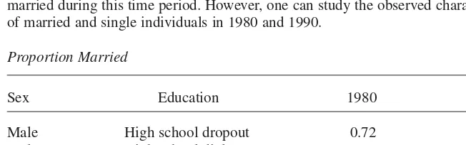
It is well known that there has been a decline in the proportion of people who are married during this time period. However, one can study the observed characteristics of married and single individuals in 1980 and 1990.
Proportion Married
Sex Education 1980 1990
Male High school dropout 0.72 0.62
Male High school diploma 0.71 0.66
Male College degree 0.73 0.72
Female High school dropout 0.68 0.62
Female High school diploma 0.73 0.69
Female College degree 0.68 0.68
Table 3
Estimates from Differenced Labor Supply Functions (Men)
WLS G2SLS UEVE WLS G2SLS UEVE
(1) (2) (3) (4) (5) (6)
Dependent Variable: Log(Annual Hours)
Log(wife’s wage) 0.180 0.253 0.232 0.005 0.074 0.001
(0.027) (0.041) (0.050) (0.026) (0.061) (0.129) Log(husband’s wage) 0.046 0.054 0.074 −0.070 −0.058 −0.001
(0.027) (0.038) (0.047) (0.024) (0.041) (0.064) Nonlabor income −0.168 −0.269 −0.282 −0.111 −0.314 −0.250
*10,000 (0.043) (0.060) (0.071) (0.046) (0.096) (0.236)
Husband and wife No No No Yes Yes Yes
indicators
Standard errors are calculated using Huber-White covariance matrix.
The table shows that the proportion married has declined for both sexes with the biggest decline for individuals with less education. Thus, it is possible that the unob-served characteristics of married people have changed over time. Because the table suggests that these changes may not be similar across groups, estimates from specifi-cations without husband and wife type controls may be biased. However, even if changes in unobservables differ across groups, the estimates from specifications with husband and wife type controls will still be consistent if unobserved changes are sim-ilar within groups across regions.
The second possibility is that even among married people, the choices of spouse have changed over time. It should be noted that certain types of changes are allowed for in the empirical work. The specification with husband and wife controls allows the composition within husband-wife groups to change while still identifying the labor supply elasticities using regional variation.
There are differences in the proportion of matches of different types between 1980 and 1990. However, these are largely explained by the fact that there are fewer matches involving high school dropouts due to the increase in educational attainment of the population. I have also done a further specification check. Rather than use the actual wage change of husbands, I calculate husband wage changes for each woman by weighting the wage changes of different types of men where the weights are deter-mined by the distribution of husband types for that type of woman in 1980. I then compare this wage change to the average wage change of husbands for that woman type (which is affected by changes in matching between 1980 and 1990). I find that the averages are almost identical. Thus, it appears that there have not been large changes in marital matching between 1980 and 1990.
2. Taxes
In the analysis so far, the wages used have been gross pre-tax wages. However, the-ory suggests that labor supply decisions should depend on marginal net after-tax wages. Modeling taxes in this context is extremely difficult to do in a rigorous fash-ion because the hours decisfash-ions of individuals should depend on the marginal tax rate at each possible level of hours that they could choose to work. The marginal tax rate at the level of hours actually worked is endogenous to the labor supply choices made (See Blundell and MaCurdy 1999; Heim and Meyer 2001 for detailed discussions about the difficulties of modeling labor supply with taxes). For these reasons, it is impractical to deal with taxes in a thorough fashion in this paper. Instead, in this sec-tion, I check whether my results are robust to using post-tax rather than pre-tax wage rates.
Individuals pay federal, state, and payroll taxes on income. I compute the marginal federal tax rate for each couple in 1979 and 1989 using the Federal Income Tax Tables for “Married Filing Jointly” with the standard deduction. Similarly, the marginal state tax rates are calculated using the state income tax rate schedules.19I add the federal and state marginal tax rates to the marginal rate from the payroll taxes to get the mar-ginal tax rate from all sources. Given that income may be misreported (to the Census
or the IRS or to both) and that complexities like itemized deductions are ignored in the calculations, the marginal tax rate facing any particular individual is an estimate of the true marginal tax rate faced. Hopefully, this source of error is largely averaged out by the grouping estimator. The marginal tax rate facing individuals averages 42 percent in 1979 and 34 percent in 1989. The decline is chiefly the result of the reduced federal tax rates implemented in the Tax Reform Act of 1986. The marginal after-tax wage rate is calculated as the wage multiplied by (1-τ) where τis the marginal tax rate.
The results using after tax wages for husbands and wives are very similar to the results when pre-tax wages are used. The G2SLS own-wage elasticity is 0.85 (0.06) for women (0.06 (0.11) when husband and wife type indicators are included); the G2SLS cross-wage elasticity for women is −0.30 (0.06) (−0.41 (0.07) when husband and wife indicators are included). The own and cross-wage elasticities for husbands are small and very similar in magnitude to the estimates using pre-tax wages. Thus, it appears that using after-tax wages instead of pre-tax wages does not change the con-clusions of the analysis.
VII. Analysis of Wages and Participation of Women
In addition to hours worked, I estimate models for the probability women participate, and the probability they work full time full year (FTFY). In this case there will be no selection bias arising from the shifting composition of women who choose to work. I report estimates from regressions where the dependent vari-ables are the proportion who participate and the proportion who work FTFY.20
A generic problem in labor supply estimation arises because the market wage is not observed for nonparticipants. I take three different approaches to imputing wages of nonparticipators. The first approach I take to this problem is to impute wages of non-participators as being equal to the average wage of non-participators in their group. This approach does not completely ignore the selection problem in that a Heckman cor-rection of the type implemented in the hours equations is consistent with this approach. Essentially, since one is using the available explanatory variables (age, edu-cation, age of spouse, education of spouse, and region) to impute wages nonparamet-rically (as the mean of wages in their group), adding any function of these variables to the wage equation as a selection correction can have no effect.
However, theory suggests that the wage offers of nonparticipators are likely to be lower than the mean wage of participators. For example, in a simple search model where individuals are homogenous, individuals who draw wage offers above the reservation wage choose to work, and individuals who draw offers below the reserva-tion wage do not work. Obviously, without making further assumpreserva-tions, one cannot ascertain the wage offers of nonparticipators, particularly when wage offer distribu-tions and the value of home time are likely to be heterogeneous. Thus, I impute wages of nonparticipators making various assumptions about the part of the distribution they
come from. I estimate the participation equations under the assumptions that nonpartici-pators have wage offers on average equal to the first percentile of wages of particinonpartici-pators in their group, the tenth percentile, the twenty-fifth percentile, and the fiftieth percentile. Third, I impute wages of nonworkers by using the wage distribution of workers who work one to thirteen weeks. Missing wages are imputed for female nonworkers in group gas the average wage of female workers in group g who work between one and 13 weeks. Juhn (1992) takes a similar approach to the problem of missing wages in her study of male participation changes. However, I have not seen this approach implemented previously to impute female wages.
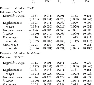
A. Results from Participation Measures
The results for the FTFYand participation analyses are in Table 4. I calculate the elas-ticities at the mean value of FTFY(0.32) and the mean value of participation (0.68). All reported specifications include husband and wife controls and use the G2SLS esti-mation method.21For both FTFYand participation, the size of the own-wage elastic-ity differs depending on how wages are imputed. The elasticities differ from about 0.4 when wages are imputed from the bottom tail of the wage distribution of participators to between 0.1 and 0.2 when wages are imputed from the mean or median of the dis-tribution. In contrast, the cross-wage elasticities are clustered around −0.20 to −0.25 for both FTFY and participation, irrespective of the method of wage imputation. These are slightly smaller than the equivalent hours elasticities. Taken together with the findings from the hours equations, there is a robust finding of negative cross-wage effects on the labor supply of wives.
VIII. Family Earnings Inequality
In this section, I use the models estimated above to examine how changes in individual wages fed through into family earnings inequality during the 1980s. The family is often considered to be the fundamental unit of society and, thus, it is important to consider the effects of wage changes and labor supply responses on changes in relative family earnings. In keeping with the rest of the paper, I will place particular emphasis on the effects of female responses to changes in husband’s wages. The first caption in Tables 5 and 6 provide an overview of female labor supply and family earnings in 1980. I begin with a sample of individuals in the 1980 Census com-posed of couples in which the husband works at some point during the year. For the purpose of exposition, I consider three types of families—both spouses with college degrees, both spouses with high school diplomas, and both spouses being high school dropouts.22I pool families into one of these three categories and I analyze the mean of each variable of interest by category.
21. As with the hours regressions, the addition of husband and wife type controls reduces the own wage elasticity but has little effect on the size of the cross-wage elasticity. The unreported UEVE estimates are similar in magnitude to the G2SLS estimates reported.
Column 1 of Table 5 shows that the mean hours of participating women are very similar across the three categories of families in 1980. However, as can be seen in the next column, participation rates increase with education level. Thus, average hours worked are also increasing with education. The final two columns show that log wages of husbands and wives increase with education with the wages of husbands being higher than the wages of wives. The first caption of Table 6 contains the average
Table 4
Estimates from Differenced Labor Supply Functions (Women)
Average 1–13 Per1 Per10 Per25 Per50
(1) (2) (3) (4) (5) (6)
Dependent Variable: FTFY
Estimator: G2SLS
Log(wife’s wage) 0.037 0.074 0.101 0.132 0.132 0.033
(0.051) (0.034) (0.028) (0.038) (0.047) (0.051) Log(husband’s −0.073 −0.074 −0.067 −0.079 −0.091 −0.073
wage) (0.034) (0.030) (0.029) (0.029) (0.032) (0.034)
Nonlabor income −0.096 −0.082 −0.066 −0.081 −0.090 −0.096 *10,000 (0.070) (0.070) (0.065) (0.069) (0.069) (0.070)
Own-wage 0.116 0.231 0.316 0.413 0.413 0.103
elasticity (0.159) (0.106) (0.088) (0.119) (0.147) (0.159) Cross-wage −0.228 −0.231 −0.209 −0.247 −0.284 −0.228
elasticity (0.106) (0.094) (0.091) (0.091) (0.100) (0.106) Dependent Variable: Participate
Estimator: G2SLS
Log(wife’s wage) 0.112 0.104 0.241 0.282 0.251 0.117
(0.047) (0.033) (0.023) (0.033) (0.041) (0.046) Log(husband’s −0.163 −0.146 −0.141 −0.164 −0.184 −0.165
wage) (0.028) (0.025) (0.022) (0.023) (0.026) (0.028)
Nonlabor income −0.344 −0.320 −0.272 −0.310 −0.328 −0.349 *10,000 (0.090) (0.085) (0.075) (0.084) (0.089) (0.089)
Own-wage 0.165 0.153 0.354 0.415 0.369 0.172
elasticity (0.169) (0.049) (0.034) (0.049) (0.060) (0.068) Cross-wage −0.240 −0.215 −0.207 −0.241 −0.271 −0.243
elasticity (0.041) (0.037) (0.032) (0.034) (0.038) (0.041)
Table 5
Actual and Counterfactual Labor Supply of Married Women by Education Group
Hours of Proportion that Log Log Husband’s Participators Participate Hoursa Wage Wage
Education (1) (2) (3) (4) (5)
Actual Means (in 1980)
High school dropout 1,455.44 0.499 726.44 1.357 1.872 High school graduate 1,480.08 0.651 963.10 1.509 2.107 College graduate 1,423.36 0.715 1,017.85 1.911 2.375 Counterfactual # 1 (Husband wage changes equal to actual changes for college graduation
High school dropout 1,558.75 0.562 876.08 1.285 1.729 High school graduate 1,703.44 0.764 1,301.19 1.510 2.009 College graduate 1,799.67 0.808 1,454.30 2.012 2.423 Counterfactual #2 (Husband wage changes equal to actual changes for college graduates) High school dropout 1,452.54 0.530 770.20 1.285 1.920 High school graduate 1,610.33 0.740 1191.20 1.510 2.155 College graduate 1,801.59 0.808 1,455.85 2.012 2.423
a. Average hours over both participators and nonparticipators.
See text and Appendix A2 for details about how the counterfactuals are implemented.
earnings of husbands and wives in each educational category. Earnings of both hus-bands and wives increase with education. Thus, assortative mating increases the absolute differences in family earnings between men of different education levels. Put another way, earnings of wives increase rather than decrease relative earnings differ-ences among men in these three types of families.
As can be seen by comparing the wages in caption two of Table 5 to those in cap-tion one, wage inequality increased for both men and women over the decade of the 1980s. In particular, there were large falls in the real log wages of men without col-lege degrees and increases in the real wages of men with colcol-lege degrees. The cross-wage elasticities estimated above suggest that wives have adjusted hours in response to these changes in relative wages. This behavioral response by wives would tend to reduce family earnings inequality. However, since wage growth of husbands and wives are correlated because of assortative mating, family earnings inequality might still have increased over this period. I examine the relative sizes of these two effects below.
First, I use the labor supply specifications for women to approximate the changes in female labor supply between 1980 and 1990.23That is, I assume each individual log
wage change equals the average log wage change of individuals of their sex in their group between 1980 and 1990. This assumption approximates the actual changes in wages that occurred between 1980 and 1990. Throughout this section, I assume that the husbands’ participation and hours decisions do not respond to changes in their wives wages. I assume these elasticities of zero rather than use the small, and impre-cise elasticities for husbands estimated in Table 3. I include a detailed description of how the predictions are carried out in Appendix A2.
The second panel in Tables 5 and 6 contain results under this counterfactual. The first column shows that the predicted hours of participating women are higher than the actual hours in 1980 for all three categories. This reflects both labor supply responses of women to changes in their own wage and husband’s wage and changes in tastes for work (captured by the group dummies in the regression). The increases are much larger for more educated women. Likewise the proportion who participate increases for all three categories, here the increase does not differ much across cate-gories. The next column contains an estimate of the average number of hours worked for each woman in the category. I calculate this as the proportion who participates multiplied by the predicted average hours of participators. Hours increase for all three categories, but the increase for the dropout group is not nearly as large as the increase for the other two groups (the percentage increase in hours is 21 percent for the dropout group, 35 percent for the high school graduates, and 43 percent for the college graduates).
Table 6
Actual and Counterfactual Earnings of Married Women by Education Group
Earnings of Earnings of Log Log Husband’s Participators Husband Earningsa Wage Wage
Education (1) (2) (3) (4) (5)
Actual (in 1980)
High school dropout 6,211.98 14,059.54 3,100.52 1.357 1.872 High school graduate 7,451.90 19,131.82 4,849.02 1.509 2.107 College graduate 10,749.62 27,195.08 7,687.13 1.911 2.375 Counterfactual #1 (Actual wage changes between 1980 and 1990)
High school dropout 6,216.75 12,217.51 3,494.09 1.285 1.729 High school graduate 8,615.58 17,442.62 6,581.10 1.510 2.009 College graduate 15,120.14 28,529.09 12,218.45 2.012 2.423 Counterfactual #2 (Husband wage changes equal to actual changes for college graduates) High school dropout 5,801.96 14,754.01 3,076.47 1.285 1.920 High school graduate 8,166.91 20,076.84 6,041.25 1.510 2.155 College graduate 15,149.99 28,538.38 12,242.58 2.012 2.423
a. Average Earnings over both participators and nonparticipators.
These labor supply changes suggest that earnings increased more for highly edu-cated women over this period. This is confirmed in the second caption of Table 6. Predicted earnings of wives in all three categories rose over the decade. High school dropout men suffered falls in real labor earnings of nearly $2,000 over the decade; the increase in their wives’ labor earnings was only $394.24Thus, the increase in female earnings offset only about one fifth of the earnings losses suffered by their husbands. On the other hand wives of college graduates had increases in real earnings of about $4,500, with their husbands having an increase of lesser magnitude. Thus, while in principle labor supply responses by wives could maintain family incomes for groups in which men have had big falls in earnings, the magnitudes of the elasticities have not been sufficient to do this in practice.
To get an idea of how much the cross-wage elasticity of women mattered in this period, I use the same model to predict outcomes under a different assumption. In this counterfactual, each woman’s log wage change equals the average log wage change of women in their group between 1980 and 1990. Each husband’s log wage change equals the average log wage change of married men with college degrees. This assumption enables one to examine how female hours and family earnings would have changed if all men had the same proportional wage change. The choice of the wage growth of college men is somewhat arbitrary. What is important is that all men are constrained to have the same log wage change.
The third captions of Tables 5 and 6 contain results from this counterfactual. As we would expect, the increased wage of husbands in this scenario leads to reduced hours and participation for the less-educated women compared to that in panel two. Consider the high school dropout family: The hours of participators average 1,455 in 1980, by 1990 these had increased to approximately 1,560. However, if the husbands of high school dropout women had the same increase in log wages over the decade as male college graduates, the hours of participators would only have been 1,450 in 1990. Thus, all of the increase in hours of participating high school dropout women between 1980 and 1990 can be accounted for by the decrease in wages of their hus-bands relative to the wages of male college graduates. Likewise, the participation rate of high school dropout women increased by approximately 0.063 between 1980 and 1990. However, if the husbands of high school dropout men had the same increase in log wages over the decade as male college graduates, the participation rate of dropout women would only have increased by about 0.031. This implies that about one half of the increase in participation of high school dropout women over the decade can be accounted for by the decline in their husbands’ wages relative to the wages of college graduate men. It appears that changes in men’s wages have had a significant effect on the labor supply decisions of their wives over this period.
The third panel in Table 6 contains predicted earnings under this counterfactual. Compared to the outcomes predicted in panel two of Table 6, we see that, for the high school dropout family, the increase in husband’s earnings is offset to some extent by the reduction in wife’s earnings. However, this is a relatively small effect—a $2,500 increase in male earnings compared to a $400 fall in female earnings. The
reducing effect of compensatory labor supply behavior is overwhelmed over this period by the inequality-increasing effect of the correlated wage growth of husbands and wives. However, it is worth noting that predicted earnings of high school dropout women in the third panel of Table 6 are similar to (actually slightly lower than) their actual earnings in 1980. This implies that none of the increase in earnings of high school dropout women over this decade would have occurred if their husbands’ wage changes were the same as the wage changes of male college graduates. Thus, while compensatory labor supply behavior of wives was insufficient to maintain the family labor earnings of low-wage men, in the absence of such behavior, the earnings of wives of low-wage men would not have increased at all.
IX. Conclusions
The large changes in relative wages that occurred during the 1980s provide fertile ground for studying the behavioral responses of married couples to the wage changes of husbands and wives. I find estimates of own-wage and cross-wage elasticities for men that are very small and the sizes of the effects are quite robust across specifications. The own-wage elasticity for women does vary across specifica-tions, probably reflecting the greater composition changes that have occurred in the female labor force over time. However, the cross-wage elasticity for women is remarkably constant across specifications and suggests a strong negative response of female labor supply to changes in their husband’s wages.25
The nonrobustness of female own-wage elasticities suggests that one must be cau-tious about drawing strong conclusions from correlations between changes over time in female wages and hours worked. New female participators may have very different skills to existing workers and changes in relative wages may reflect these composition changes to some degree. Participation changes among males have been much smaller in recent decades and thus changes in male wages may suffer less from such biases. For this reason, it is not so surprising that female labor supply reactions to male wage changes are much more stable across specifications than are own-wage elasticities.
Similar caution is required to interpret the correlations between changes in hus-bands wages and wife’s labor supply. During the 1980s the labor supply of wives of high-wage men increased more than the labor supply of low-wage men. This occurred despite the greater wage increases of high-wage men. One might conclude from this correlation that the cross-wage elasticity of women is positive. However, once one accounts for the correlations in wage changes of spouses that results from assortative mating, the estimates suggest a negative economically significant cross-wage elastic-ity. Moreover, this elasticity is stable across numerous specifications.
Family labor supply behavior determines how changes in individual wage rates translates into family earnings changes. The responses of women to changes in their husbands wages attenuated somewhat the increases in individual wage inequality at the family level. The results suggest that the earnings of the wives of low income men
would actually have fallen over the decade if women’s labor supply did not respond to changes in their husbands’ wages. However, assortative mating implies that wage changes of husbands and wives are correlated and so family earnings inequality still grew during the decade of the 1980s.
Appendix A1
The UEVE Estimator
Consider the regression at the level of population means (the means for all members of the underlying population who are in that group):
* *
y
∆ =∆x β ε+
Here, y* refers to the mean of ywithin each group and x* is a vector of the means of
x. However, one calculates from the data the sample means xrand yrrather than x* and
y*. Assume that sampling error has the following structure:
*
The WLS estimator on the group means is biased in this errors-in-variables context. Define N as the number of groups and k as the number of right hand side variables. From results in Deaton (1985) and Devereux (2003), one can derive that the UEVE estimator below is approximately unbiased and is consistent as the number of groups goes to infinity:
( ) ( )
x N k y N k
βUEVE=`∆ ∆xrl r-2 - -1 Σtj-1_∆ ∆xrl r-2 - -1 σti
The variances and covariances of measurement error are estimated by their empiri-cal counterparts. I estimate the elements of σtby calculating the covariance between log hours and each of the x variables in each group in each time period. Likewise, I calcu-late the rows and columns of Σt by estimating the variances and covariances of the x
variables within group in each year.26In both cases, I take the weighted average of the covariances across groups and years and divide by the average number of observations in each group. I weight the regressions by multiplying each sample mean by the square root of the number of observations in that group. Equivalently, the variances and covariances are multiplied by the average number of observations per group.
The robust standard errors are calculated using the following variance-covariance matrix:
*( /( ))*
where e is the vector of residuals. It is assumed in calculating the variance-covariance matrix that Σand σare known (unsurprisingly, given these are calculated using over a million observations in each year, accounting for sampling error in the variance esti-mates has negligible effects on the standard errors).
Appendix A2
Counterfactual Hours and Earnings
I begin with a sample of individuals in the 1980 Census composed of couples in which the husband works at some point during the year. Wage changes are unavailable at the individual level and so I predict hours and earnings under the assumption that wage changes are the same for all members of the same group. Specifically, I use two dif-ferent counterfactuals.
Counterfactual 1
Each individual log wage change equals the average log wage change of individuals of their sex in their group (same age, education, and census division) between 1980 and 1990. This assumption approximates the actual changes in wages that occurred between 1980 and 1990.
Counterfactual 2
Each woman’s log wage change equals the average log wage change of women in their group between 1980 and 1990. Each husbands log wage change equals the average log wage change of married men with college degrees.
Predicting Hours
I begin by using the sample of marriages in which both individuals participate and predict the hours of women conditional on working. The estimating equation relates changes in log hours to changes in the log wages of each spouse (The actual specifi-cation used is the linear labor supply equation estimated by G2SLS. The estimates are reported in Table 2, Column 5.) Let ∆ˆ log hfbe the predicted change in log hours from the regression, and let εbe the residual from the regression. The expected value of log hours of each wife (Elog hf) under either counterfactual equals her log hours in 1980 (log hf80) plus the predicted change in log hours (∆ˆ log hf). Likewise the expected value of hours for each wife under either counterfactual, is calculated as follows:
( ) ( )
E hf =Eexp logh80f +∆tloghf+ε
This implies that E(hf) =hf80*exp(∆ˆ log hf)* Eexp(ε)
female participator under each counterfactual, I can take means within each group to find the average hours of participators under each scenario. I also estimate the propor-tion of each educapropor-tion group that works in the counterfactual regimes using the linear probability model estimates in Column 1, Table 4. Then, by definition, the average hours worked over all women in the group (including participators and nonparticipators) equals the average hours of participators multiplied by the proportion who participate.
The equivalent exercise is carried out for female earnings. Here I make use of the fact that log(hf wf) =log(hf) + log(wf). Thus, the predicted change in log earnings equals the predicted change in log hours plus the change in the log wage. Given the predicted change in log earnings, I proceed to predict actual earnings in an equivalent manner to that with hours.
Table A1
Deviation in log Wage Change from Average Log Wage Change in Region
1 2 3 4 5 6 7 8 9
East West East West
New Middle North North South South South
Age/Education England Atlantic Central Central Atlantic Central Central Mountain Pacific
Women
21-30/HSDO −0.06 −0.08 −0.10 −0.11 −0.09 −0.08 −0.10 −0.07 −0.10
31-40/HSDO −0.09 −0.08 −0.08 −0.06 −0.08 −0.03 −0.10 −0.05 −0.11
41-50/HSDO −0.07 −0.07 −0.05 −0.06 −0.07 −0.06 −0.06 −0.01 −0.09
51-60/HSDO −0.09 −0.07 −0.05 −0.03 −0.07 0.01 −0.08 −0.07 −0.07
21-30/HSG −0.01 −0.03 −0.04 −0.03 −0.02 −0.03 −0.04 −0.03 −0.01
31-40/HSG 0.01 0.01 0.02 0.01 0.02 0.01 0.02 0.00 0.01
41-50/HSG 0.04 0.00 0.01 0.01 0.03 0.03 0.03 0.01 0.02
51-60/HSG −0.03 −0.01 0.00 −0.01 −0.02 0.01 0.03 −0.03 −0.02
21-30/CG 0.06 0.08 0.08 0.04 0.06 0.03 0.09 0.08 0.08
31-40/CG 0.02 0.05 0.08 0.07 0.06 0.06 0.09 0.10 0.06
41-50/CG 0.02 0.09 0.07 0.09 0.07 0.09 0.07 0.05 0.07
51-60/CG −0.03 −0.03 0.06 0.05 0.04 0.08 0.05 0.02 0.00
Men
21-30/HSDO −0.03 −0.04 −0.13 −0.10 −0.04 −0.08 −0.11 −0.10 −0.08
31-40/HSDO −0.06 −0.10 −0.13 −0.08 −0.05 −0.08 −0.11 −0.09 −0.14
41-50/HSDO −0.03 −0.05 −0.04 −0.06 −0.05 −0.02 −0.07 −0.09 −0.16
51-60/HSDO −0.04 −0.04 −0.01 −0.02 −0.06 0.01 −0.07 −0.05 −0.08
21-30/HSG 0.05 −0.03 −0.08 −0.05 −0.02 −0.07 −0.05 −0.04 −0.02
31-40/HSG −0.03 −0.06 −0.05 −0.05 −0.04 −0.04 −0.04 −0.03 −0.03
41-50/HSG −0.02 0.00 0.03 0.02 0.02 0.04 0.03 0.01 0.00
51-60/HSG 0.01 0.03 0.04 0.01 0.00 0.05 0.04 0.01 0.02
21-30/CG 0.13 0.15 0.12 0.13 0.11 0.12 0.11 0.10 0.13
31-40/CG 0.01 0.06 0.11 0.09 0.05 0.11 0.12 0.11 0.10
41-50/CG −0.01 0.06 0.12 0.10 0.08 0.10 0.13 0.10 0.07
References
Angrist, Joshua. 1991. “Grouped-Data Estimation and Testing in Simple Labor-Supply Mod-els.” Journal of Econometrics47 (Feb/March):243–66.
Blundell, Richard, Alan Duncan, and Costas Meghir. 1998. “Estimation of Labour Supply Responses using Tax Policy Reforms.” Econometrica66(4):827–61.
Blundell, Richard, Pierre-Andre Chiappori, Thierry Magnac, and Costas Meghir. 2001. “Col-lective Labor Supply: Heterogeneity and Non-Participation.” Institute of Fiscal Studies, WP01/19.
Blundell, Richard, and Thomas MaCurdy. 1999. “Labor Supply: a Review of Alternative Approaches.” In Handbook of Labor EconomicsVolume 3A, ed. Orley Ashenfelter and David Card. Amsterdam: Elsevier Science.
Borjas, George, and Valerie Ramey. 1995. “Foreign Competition, Market Power, and Wage Inequality.” Quarterly Journal of Economics110(4):1075–1110.
Bound, John, David Jaeger, and Robert Baker. 1995. “Problems with Instrumental Vari-ables Estimation When the Correlation between Instruments and the Endogenous Explanatory Variable is Weak.” Journal of the American Statistical Association
90(43):443–50.
Bumpass, Larry, and James Sweet. 1989. American Families and Households. New York: Russell Sage Foundation.
Chiappori, Pierre-Andre. 1988. “Rational Household Labor Supply.” Econometrica
56(1):63–90.
———. 1992. “Collective Labor Supply and Welfare.” Journal of Political Economy
100(3):437–67.
Deaton, Angus. 1985. “Panel Data from a Time Series of Cross-Sections.” Journal of Econo-metrics30: 109–126.
Devereux, Paul. 2003. “Changes in Male Labor Supply and Wages.” Industrial and Labor Relations Review56(3): 409– 428.
———. 2003. “Improved Errors-in-Variables Estimators for Grouped Data.” Working Paper.
Gosling, Amanda, and Thomas Lemieux. 2001. “Labor Market Reforms and Changes in Wage Inequality in the United Kingdom and the United States.” National Bureau of Eco-nomic Research Working Paper number 8413.
Gronau, Reuben. 1974. “Wage Comparisons—A Selectivity Bias.” Journal of Political Econ-omy82(6):1119–43.
Hausman, Jerry, and Paul Ruud. 1984. “Family Labor Supply with Taxes.” American Eco-nomic Review74(2):242–48.
Heckman, James. 1979. “Sample Selection Bias as a Specification Error.” Econometrica
47(1): 153–62.
Heim, Bradley, and Bruce Meyer. 2001. “Structural Models of Labor Supply in the Presence of Nonlinear Budget Sets.” Working Paper.
Hyslop, Dean. 2001. “Rising U.S. Earnings Inequality and Family Labor Supply: The Covari-ance Structure of Intrafamily Earnings.” American Economic Review91(4):755–77. Imbens, Guido, Donald Rubin, and Bruce Sacerdote. 2001. “Estimating the Effect of
Unearned Income on Labor Supply, Earnings, Savings and Consumption: Evidence from a Sample of Lottery Players.” American Economic Review91(4):778–94.
Juhn, Chinui. 1992. “Decline of Male Labor Force Participation: The Role of Declining Mar-ket Opportunities.” Quarterly Journal of Economics107(1):79–121.
Juhn, Chinui, and Dae Kim. 1999. “The Effects of Rising Female Labor Supply on Male Wages.” Journal of Labor Economics15(1):23–48.