Evidence from Women Seeking Fertility
Services
Julian P. Cristia
a b s t r a c t
Estimating the causal effect of a first child on female labor supply is complicated by the endogeneity of fertility. This paper addresses this problem by focusing on a sample of women from the National Survey of Family Growth (NSFG) who sought help to become pregnant. After a certain period, only some of these women gave birth. Results using this strategy show that having a first child younger than one year old reduces female employment by 26 percentage points. These estimates are close to OLS estimates from census data and to those from OLS and fixed-effects models on NSFG data.
I. Introduction
Estimating the effect of fertility on female labor supply has been a longstanding problem in economics. Knowing how families optimize their labor sup-ply decisions in response to the arrival of a child is important for several reasons. First, it is interesting to know how much of the increase in female labor supply since the World War II can be explained by delayed childbearing and reduced fertility (Goldin 1990). Second, some researchers believe that the interruption of work attrib-utable to childbearing is responsible for a significant proportion of the male-female wage gap (Fuchs 1989; Korenman and Neumark 1992), and the size of the impact of
Julian Cristia is a research fellow at the Office of Evaluation and Oversight of the Inter-American Development Bank. The author wishes to thank Julio Caceres Delpiano, Mark Duggan, Eugenio Giolito, Amy Harris, Sandra Hofferth, Arlene Holen, Beomsoo Kim, Noah Meyerson, Reed Olsen, Caroline Polk, Seth Sanders, Jonathan Schwabish, Michael Simpson, John Skeen, Julie Topoleski, two referees, and seminar participants at University of Maryland, Congressional Budget Office and the 2007 Population Association of America Meetings for invaluable comments and suggestions. The data used in this article can be obtained beginning January 2009 through December 2012 from Julian Cristia, 1350 New York Avenue, N.W., Stop B760, Washington, D.C. 20577, e-mail: jcristia@iadb.org. The views expressed in this paper are those of the author only and are not necessarily the views of the Inter-American Development Bank, its board of directors, nor the countries they represent. [Submitted April 2007; accepted August 2007]
ISSN 022-166X E-ISSN 1548-8004Ó2008 by the Board of Regents of the University of Wisconsin System
childbearing on female labor supply is an important variable in that calculation. Third, if declines in labor supply after childbearing correspond to increases in child-care time, then knowing the effect of childbearing on female labor supply will pro-vide information about time inputs invested in the child (Blau and Grossberg 1992). Finally, and above all, economists have been interested in this question from a basic desire to know the quantitative importance of various determinants of female labor supply.
Hundreds of published studies have examined the relationship between fertility and female labor supply. However, as Browning (1992) notes in his literature review on this topic, ‘‘Although we have a number of robust correlations, there are very few credible inferences that can be drawn from them’’ (p. 1435). The key problem researchers face is that the fertility decision may be endogenous; therefore, the strong negative correlations found between different measures of fertility and female labor supply cannot be interpreted as evidence of causal effects.
To overcome the type of criticism highlighted by Browning (1992), two strategies have exploited exogenous changes in family size in order to estimate the effect of fertility on female labor supply. The first strategy (Rosenzweig and Wolpin 1980; Bronars and Grogger 1994; Jacobsen, Pearce, and Rosenbloom 1999) used the fact that twins in the first birth represent an exogenous change in family size in order to estimate the effect of having a second child. The second strategy (Angrist and Evans 1998) exploited parental preferences for mixed-sex siblings in order to esti-mate the effect of a third or higher order child. For a sample of couples with at least two children, they instrumented further childbearing (having more than two children) with a dummy variable for whether the sexes of the first two children match.
Still, the question of how a first child affects female labor supply has not been pre-viously addressed with a strategy that directly tackles the problem of the endogeneity of fertility. It could be argued that the effect of having a first child is the most im-portant one, given that it applies to a vast majority of women, whereas the effect of having a second or higher order child only applies to a smaller subset of women.1 This paper examines a situation in which the problem of the endogeneity of fer-tility is minimized. In particular, it focuses on a sample of childless women who sought help with achieving pregnancy. At the time of seeking help, all of the women wanted to have a child; after a certain period, some of them gave birth, and others did not. Then, employment rates of women in the ‘‘treatment’’ group (those who gave birth to a child) are compared to employment rates from those in the control group (those who did not give birth).2
The contribution of this paper is that while analysis of twins and the preference for mixed-sex siblings strategy, under certain conditions, can be used to identify the ef-fect of a second or higher order child, the estimation strategy pursued here is able to identify the effect of a first child on female labor supply.
My work is also related to studies that exploited the stochastic component of fer-tility to estimate the effect of changing the timing of childbearing on long-run earn-ings. Hotz, McElroy, and Sanders (2005) used miscarriage in a woman’s first
1. In the 1990 census, among women aged 45 to 55, 89.0 percent had at least one child, whereas 78.3 per-cent had at least two and 50.4 perper-cent had at least three children.
pregnancy as an instrument to estimate, for a sample of teen mothers, the effect of delayed childbearing on annual hours and earnings. Miller (2005) focused on the same question for an older group of women and instrumented age at first birth using miscarriages, contraception failures, and the lag between first attempt to conceive and birth.
The strategy used in this analysis tackles the problem of fertility being an endog-enous variable because all women wanted to have a child at the time they sought help. Early success in fertility treatment, however, is not expected to be completely random. Still, I provide several pieces of evidence suggesting that the strategy con-sistently estimates the parameter of interest. First, following Heckman and Hotz (1989), I find that women’s employment, during months prior to seeking help becom-ing pregnant, is uncorrelated with subsequent fertility. Second, estimates of the pa-rameter of interest are very robust to the set of covariates added to the main regression. Third, observable characteristics of the sample of childless women that sought help achieving a first pregnancy are quite similar to those of women who have their first child after age 18.
Using the exogenous assignment of children to women who seek help achieving pregnancy, I estimate that having a first child younger than one year old reduces fe-male employment by 26 percentage points. These estimates are close to ordinary least squares (OLS) and fixed-effects estimates obtained from panel data from the National Survey of Family Growth (NSFG). They also are close to OLS estimates obtained using similarly defined samples from the 1980 and 1990 censuses. This finding is important because previous studies that dealt with the endogeneity of the fertility decision typically provided smaller estimated effects than studies that as-sumed exogenous fertility. Finally, I provide evidence of a reduction in the estimated short-term impact of childbearing on female labor supply of 40–50 percent between 1980 and 1990.
II. Background: The Reproductive Process
and Infertility
Healthy couples having intercourse regularly have only a 20 percent chance of conceiving during a month. This statistic implies that about 26 percent of healthy couples will not have conceived after six months of unprotected sex; this number falls to about 7 percent after 12 months. As a result, couples are recommen-ded to start fertility testing and treatment only after 6–12 months of trying to con-ceive without success. The medical community typically defines a couple as infertile if they have not conceived after 12 months of unprotected sex.3The National Center for Health Statistics (NCHS) estimated that in 1995, there were 2.1 million infertile married couples in the United States and that 6.1 million women aged 15–44 had an impaired ability to have children.
Medical researchers have identified a number of factors that affect the fertility prognosis of a couple. The woman’s age, education, smoking status, consumption
of recreational drugs, and obesity, as well as sexual frequency, are important predic-tors of the probability of conception (Dunson, Baird, and Colombo 2004).
Given the stochastic nature of the reproduction process, physicians usually start treatment with simple and inexpensive procedures (for example, advice and testing) and only start using more invasive and expensive procedures as the simple proce-dures prove unsuccessful. For example, physicians typically recommend in vitro fer-tilization methods only after all other options have been exhausted or if they strongly believe that less invasive procedures will be unsuccessful.
III. Data
This paper uses data from the National Survey of Family Growth (NSFG), a survey conducted by the National Center of Health Statistics in 6 cycles (1973, 1976, 1982, 1988, 1995, and 2002). Cycles 1–5 were conducted at the homes of a nationally representative sample of women aged 15–44. Cycle 6 also sampled men aged 15–44. The main purpose of the surveys was to provide reliable national data on marriage, divorce, contraception, fertility, and the health of women and infants in the United States.
Data from the NSFG Cycle 5 were chosen for this paper because they provide ret-rospective information about births, pregnancies, use of fertility services, demo-graphic characteristics, and the complete work history for each individual.4 In particular, the data provide the month in which each woman sought help for the first time to achieve pregnancy, information that is critical for the strategy pursued in this paper. Other important variables included are age, race, ethnicity, educational attain-ment, school enrollattain-ment, and smoking history. The survey also reports data on each full-time and part-time employment spell.
The NSFG Cycle 5 used a multistage sampling design that oversampled Hispanic and black women. It took place between January and October 1995, and the response rate was 79 percent. A total of 10,847 women were interviewed.
Data on fertility and employment are collected retrospectively. Although this type of design has limitations, Teachman, Tedrow, and Crowder (1998) found the NSFG Cycle 5 data to be of high quality. They concluded that the employment information matches the Current Population Survey (CPS) data reasonably well, although the data on employment spells have not been validated using external records.
IV. Empirical strategy, Parameter of Interest, and
Sample Construction
A. Empirical Strategy
A hypothetical social experiment aimed at estimating the causal effect of childbear-ing on female labor supply would recruit women who wanted to have a child and then assign a child to women in the treatment group while not assigning a child to
a second group (the control group). Given the stochastic nature of conception, this type of experiment can be approximated. To start, we need a group of women who want to conceive a baby. Second, some of the women should receive babies in a way that is uncorrelated with baseline employment. Third, we need to observe female la-bor supply for both groups of women for a certain time after they start trying to con-ceive.
I aim to mimic this hypothetical social experiment and fulfill the three aforemen-tioned conditions by focusing on the following situation. I construct a sample of women who sought help to have a first child (called the HELP sample). Because women in this sample sought help to achieve pregnancy at different points in time, I normalize time by the month in which they sought help for the first time (denoted as Month 0). Next, I classify the women according to whether they had given birth to a child by Month 21. In this way, I obtain two groups of women: treatment and control. Finally, I compare employment rates of the two groups of women in Month 21 to estimate the causal effect of having a first child younger than one year old on female labor supply.
I compare employment in Month 21 instead of other months for the following rea-sons. First, at this time, 97 percent of babies born are currently younger than one year old, making the definition of the treatment effect more precise. Second, using a lon-ger horizon could allow some women in the treatment group to have additional chil-dren, which would complicate the analysis.6Third, as time since women sought help increases, those who are unsuccessful at conceiving may adopt a child. Finally, look-ing at a shorter time span, it is more plausible that the women received similar types of fertility treatments (for example, in vitro fertilization treatments typically are not considered an option in the first 12 months after seeking help achieving pregnancy). The identifying assumption under this empirical approach is that the counterfac-tual average employment level of mothers in a month (relative to the month in which they sought help) can be estimated by the average employment of childless women in that month. Using this same data, and identifying assumption, other treatment effects can be estimated aligning mothers by their month of birth and estimating their coun-terfactual employment level using information on childless women. However, the empirical approach based on classifying women by their fertility status in Month 21 is followed due to reasons mentioned above and also because of the transparency of this approach and the ability to easily compare its estimates to those from approaches that do not deal with the endogeneity of fertility.
A potential problem with this empirical strategy arises if women in the control group adopt a child, start cohabitating with, or marry someone with children. In the treatment evaluation literature, this behavior is denoted as ‘‘substitution bias,’’ and it represents a situation in which control group members receive close substitutes for the treatment in question (see Heckman and Smith 1995, pp. 22–24). In the con-text of this paper, treatment is defined as having a biological child, and a close sub-stitute is adopting one (or acquiring a stepchild). Even though substitution bias can
5. To be precise, this experiment estimates the effect of having a child on female labor supply for women who wanted to have a child, not for all women.
be a substantial problem in certain social experiments, it is minimal in this case. Only 2.7 percent of women in the control group adopted or acquired a stepchild in the 21 months after they sought help to become pregnant (and only 0.5 percent in the treatment group did so). Thus, we should expect a small downward bias in the esti-mated impact due to the higher likelihood of adoption in the control group.
B. Parameter of Interest
In this study, the parameter of interest is the average impact of having a first child younger than one year old on female labor supply for women who want to have a child. Note that the study does not provide an estimate of the effect of having a first child for women whose child is unwanted. All the same, the parameter of interest applies to a fairly large population. Henshaw (1998), using data from the NSFG Cycle 5, found that 69 percent of births were planned among women aged 15–44 in 1994.
Throughout this study, I focus only on the short-term effects of having a first child (specifically, the effect of having a child younger than one year old). It is clear that other treatment effects are worthy of attention; however, for reasons already discussed, the strategy used in this study is best suited for estimating this treatment effect.
Finally, an estimate of the impact of having a first child younger than one year old is important for a number of reasons. First, as mentioned above, this effect applies to a much wider population than estimates that focus on the effect of a second or higher order child. Second, the consensus is that the short-term effects of childbearing on female labor supply are substantially larger than the long-term effects (Browning 1992). Thus, knowing the short-term effects is useful because it gives an upper bound for the long-term effects. Third, Shapiro and Mott (1994) provided strong evidence that labor force status following the first birth is an important predictor of lifetime work experience. This finding implies that changes in the estimated short-term im-pact of having a first child on female labor supply could predict a substantial change in total lifetime work experience for women. Finally, using this empirical strategy I can compare the estimated effects obtained when tackling the endogeneity problem (that is, using the HELP sample) with estimates from strategies that do not tackle this problem (for example, OLS on census data).
C. Sample Construction
The HELP sample includes childless women who sought help with becoming preg-nant when aged 19–38. The age restriction in the sample is due to two reasons. First, the results obtained in the HELP sample are compared to those from census and NSFG samples, and an age restriction is needed in constructing these samples in or-der to select women at risk of having children. Second, work information is only reported for women aged 18 and older, and employment status one year before seek-ing help is needed to check past employment levels between the treatment and con-trol groups. Also, women that sought help in the 21 months preceding the interview are dropped from the HELP sample, because it is not possible to observe their child and labor status at this time.
medical provider to talk about ways to help you become pregnant?’’ In turn, these women were asked ‘‘In what month and year did you make your first visit to seek medical help for becoming pregnant?’’ This last question allows one to identify a point in time for each woman in which she wanted to have a child and this piece of information is used to exploit exogenous shocks to fertility in this setting. More-over, the wording of the first question allows identification of a large group of women who wanted to have children but were unsuccessful after trying for certain time. Women who only talked to their medical provider about help with becoming preg-nant (as opposed to those that actually received fertility treatments) are included in the HELP sample. This explains why, as it will be seen later, women in the HELP sample are fairly representative of women who have their first child when aged 19–38.7
Table 1 presents the algorithm used in order to construct the HELP sample. The table shows that only 499 observations are included in the empirical analysis, a fact that may seem to be a limitation for the study. As shown in Section V, however, I precisely estimate the relevant coefficient of the effect of having a first child on female labor supply.
Table 1
Algorithm for Constructing the HELP Sample
Step
Number of Remaining Observations
1. Start with the whole NSFG sample. 10,847
2. Drop women who did not seek help to get pregnant. 895
3. Drop women who sought help for the first time less than 21 months prior to the interview.
788
4. Drop women who were younger than age 19 or older than age 38 when seeking help for the first time.
745
5. Drop women who had already a child when seeking help for the first time.
553
6. Drop women who had adopted or acquired a stepchild when seeking help for the first time.
536
7. Drop women who were pregnant at some point of the month in which they sought help for the first time.a
500
8. Drop a woman with missing information in the insurance coverage variable.
499
a. This group could include women who became pregnant right after seeking help for the first time (which occurred in the same month), or who were pregnant at the time when they sought help but did not know it. In fact, 23 of the 36 women who reported being pregnant in the same month they first sought help became pregnant in that month or in the previous one.
The basic empirical strategy of this paper is based on comparing women in the HELP sample who had had a baby by Month 21 with those who did not. To identify the two groups of women, I define a variable calledAnyChildren21which equals one if the woman had a baby by Month 21 and zero if she did not. In this setting, women from the HELP sample for whom AnyChildren21 equals one are in the treatment group and those for whomAnyChildren21equals zero are in the control group.
The plausibility of the proposed empirical strategy rests on the assumption that treatment is not correlated with baseline labor supply. However, in some scenarios this assumption will not hold. For example, if women married to high earner men have a higher probability of success (through access to better fertility treatments) and tend to have a lower attachment to the labor market (due to an income effect), then the effect of fertility on female labor supply will be underestimated. To assess the plausibility of the empirical strategy, I take two steps. First, I compare summary statistics on covariates for the treatment and control groups in order to check for evidence of selection. Clearly, it is not possible to check for selection on unobserv-able factors, but lack of evidence of selection on observunobserv-able factors gives assurance that treatment can be taken as exogenous to baseline labor supply.8Second, I com-pare employment rates for the treatment and control groups prior to seeking help (the results are presented in Section VI).
Descriptive statistics for women in the treatment and control groups are presented in Table 2. In the NSFG Cycle 5, respondents were asked about all of their employ-ment spells, and I use those responses to construct four employemploy-ment variables. The variablesEmployed21andEmployed0are dummy variables that equal one if the re-spondent was employed in Months 21 and 0, respectively. Similarly,Employed_12
represents labor status in Month –12 (that is, 12 months before the woman sought help for the first time). Finally,Experience0corresponds to the number of years of work experience accumulated since age 18 up to Month 0.
Although employment rates in Months 0 and –12 are similar between the treat-ment and control groups, employtreat-ment rates differ by 25.3 percentage points in Month 21. Moreover, observable characteristics in Month 0 for treatment and control women are quite similar. As shown in Table 2, differences in means of key covariates between the treatment and control groups are only statistically significant at the 5 percent significance level for the dummy variables for Hispanic and smoking.
Consistent with these results, Table 3 presents linear probability estimates of the effect of selected covariates on fertility at Month 21 and shows that smoking and His-panic ethnicity are significant predictors of fertility success. However, the adjusted
R2is only 4.3 percent, which means that much of the variation in the fertility variable remains unexplained in the model.
A potential caveat for the strategy pursued in this paper is that, as many times is the case in social and medical experiments, the sample involved in the experiment may not be representative of the population of interest. To gauge the potential sever-ity of this problem, Table 4 compares descriptive statistics of women in the HELP sample with those of women in the NSFG who had at least one child. For women in the HELP sample, time-varying variables (Age,Year,Employed_12,Education,
Married,Smoke) are measured at the time they first sought help achieving pregnancy, whereas for NSFG women the variables are measured at the time of first birth. The second column of Table 4 presents statistics for the set of women in the NSFG who had their first child when aged 19–38 because that is the age range of women in the HELP sample.
Comparing the second and third column of Table 4, we see that women in the HELP sample tend to be older and more educated and to have higher employment,
Table 2
Employed21(¼1 if employed in Month 21)
0.798 0.624** 0.877
Employed0(¼1 if employed in Month 0)
0.862 0.881 0.853
Employed_12(¼1 if employed in Month —12)
AnyOtherChildren21(¼1 if had adopted or stepchildren in Month 21)
0.020 0.005 0.027
Age0(age in Month 0) 26.3 (4.3) 25.9 (4.7) 26.5 (4.1)
Year0(year in Month 0 normalized as 1970¼0)
14.7 (5.7) 15.0 (6.1) 14.5 (5.5)
Education0(years of education in Month 0)
13.6 (2.5) 13.8 (2.6) 13.5 (2.4)
Hispanic(¼1 if Hispanic) 0.069 0.113* 0.050
Black(¼1 if black) 0.087 0.078 0.091
Married0(¼1 if married in Month 0) 0.884 0.884 0.884
Smoke0(¼1 if smoked in Month 0) 0.370 0.286* 0.408
InsuranceCovered(¼1 if insurance covered fertility treatments)
0.789 0.792 0.787
N 499 164 335
* Significantly different from the control group at the 5 percent level. ** Significantly different from the control group at the 1 percent level. a. Mother and childless refers to own biological children.
marriage, and smoking rates than women from the NSFG that were aged 19–38 when they had their first child. A lower proportion of HELP women are Hispanic or black than NSFG women. Still, basic statistics for the HELP sample are not very different from those of their counterparts in the NSFG. The last column of Table 4 presents basic statistics for the HELP sample when observations are reweighted to match the distribution by age and year groups for 19- to 38-year-old NSFG women with children. This adjustment makes the proportion of Hispanic and black women similar across the two samples and brings mean education closer.
V. Results
This section presents the main results of the empirical analysis. In es-sence, I compare employment rates in Month 21 for treatment and control women in the HELP sample. The econometric model is represented by this simple OLS equa-tion:9
Employed21i¼a+bAnyChildren21i+gXi+ui
ð1Þ
Table 3
Linear Probability Estimates. Predicting Fertility using Selected Covariates
Independent variable
Dependent variable:
AnyChildren21 Coefficient (Standard Error)
Age0 20.012 (0.012)
Year0 0.007 (0.005)
Smoke0 20.102 (0.046)
Education0 0.013 (0.010)
Hispanic 0.193 (0.082)
Black 20.054 (0.067)
Married0 20.015 (0.051)
InsuranceCovered 0.024 (0.054)
Experience0 20.005 (0.011)
Constant 0.394 (0.244)
Adjusted R2 0.043
P-value ofF-test of joint significance 0.004
N 499
Note: Regression run on the HELP sample. The mean ofAnyChildren21is 0.312.
where the vector of covariates includes black and Hispanic dummy variables; an in-dicator for insurance coverage of fertility treatments; year in which the women sought help for the first time; and the following variables measured in Month 0: age, smoking status, years of education, and accumulated work experience (in years). To gauge the potential importance of the problem of not having data on certain variables that may be simultaneously correlated with conception and labor supply, I run a number of regressions including separate sets of covariates. If the results were sensitive to the set of covariates added to the regression, they would raise some doubts as to whether the identification strategy consistently estimates the parameter of interest. Table 5 presents the regression results.
In the model that includes all covariates (Column 4), I estimate that having a first child younger than one-year-old decreases female employment by 25.7 percentage
Table 4
Comparison of HELP Sample with Childbearing Women in the NSFG
Mean (Standard Deviation)
Education 12.3** (2.6) 12.8** (2.5) 13.6 (2.5) 13.1 (2.4)
Hispanic 0.125** 0.112** 0.069 0.098
Black 0.150** 0.110 0.087 0.112
Married 0.702** 0.782** 0.884 0.857
Smoke 0.336 0.329 0.370 0.420
N 6,911 5,150 499 499
* Significantly different from the HELP sample at the 5 percent level. ** Significantly different from the HELP sample at the 1 percent level. Note: NSFG: National Survey of Family Growth.
a. Variables in Columns 2 and 3 are measured at the month in which the women gave birth to their first child (except forEmployed_12). Variables in Columns 4 and 5 are measured in the month in which they first sought help becoming pregnant (except forEmployed_12).
b. This sample is constructed by selecting from the NSFG sample all women who had at least one child. c. Includes all women in the NSFG sample who gave birth their first child when aged 19 to 38. d. Observations are reweighted to match the age and year distribution in the sample of NSFG women whose first birth occurred when aged 19 to 38.
Table 5
Linear Probability Estimates. Impact of a First Child on Employment
Dependent variable:Employed21Coefficient (Standard Error) Independent
variable (1) (2) (3) (4) (5) (6)
AnyChildren21 20.253 (0.045)
20.254 (0.044) 20.261 (0.043) 20.257 (0.041) 20.277 (0.046) 20.820 (0.254)
AnyChildren21* Age0 — — — — — 0.011 (0.011)
AnyChildren21* Year0 — — — — — 0.019 (0.008)
Age0 — 0.007 (0.005) 0.000 (0.005) 20.051 (0.011) 20.062 (0.011) 20.056 (0.011)
Year0 — 0.010 (0.004) 0.010 (0.004) 0.010 (0.003) 0.012 (0.004) 0.003 (0.004)
Smoke0 — — 20.045 (0.042) 20.035 (0.037) 20.025 (0.043) 20.033 (0.036)
Education0 — — 0.021 (0.007) 0.023 (0.007) 0.029 (0.008) 0.023 (0.007)
Hispanic — — 20.131 (0.071) 20.081 (0.067) 20.049 (0.074) 20.093 (0.066)
Black — — 0.014 (0.050) 0.011 (0.050) 20.119 (0.075) 0.008 (0.050)
Married0 — — — 20.050 (0.036) 20.107 (0.044) 20.065 (0.036)
InsuranceCovered — — — 0.082 (0.041) 0.153 (0.051) 0.071 (0.040)
Experience0 — — — 0.059 (0.010) 0.067 (0.011) 0.059 (0.010)
Constant 0.877
(0.019)
0.563 (0.126) 0.459 (0.156) 1.349 (0.205) 1.439 (0.224) 1.592 (0.211)
Adjusted R2 0.085 0.119 0.147 0.257 0.290 0.283
N 499 499 499 499 499 499
Note: Regressions run on the HELP sample. Regression 5 observations are weighted to match the age and year distribution in the sample of NSFG women whose first birth occurred when aged 19 to 38. The mean ofEmployed21using NSFG weights is 0.798 (0.771 for the reweighted sample). NSFG: National Survey of Family Growth.
The
Journal
of
Human
points. The results indicate that the estimated impact is remarkably robust to the set of covariates included in the regression. In particular, the estimated effect in a model with no covariates (Column 1) is –0.253. That is, including the entire set of covari-ates, the estimated coefficient changes by just 0.4 percentage points, or 1.6 percent of the estimated impact. The corresponding marginal effects estimates from a logit model with no covariates are –0.253 and increase to –0.288 when all covariates are included.10
Column 5 presents linear probability estimates when observations are reweighted to match the age-year distribution for the sample of mothers in the NSFG who gave birth to their first child when aged 19–38. The estimated impact is slightly higher than the one obtained from original NSFG weights (–0.277 versus –0.257). In Col-umn 6, the model is augmented to check for varying treatment effects by age of mother and year in which she sought help with achieving pregnancy. The results sug-gest that the short-term effects of childbearing have substantially decreased over time (this issue is examined more deeply in Subsection VII.B). Also, there is some evi-dence that the treatment effect may be smaller for older women though the point es-timate is not significantly different from zero.
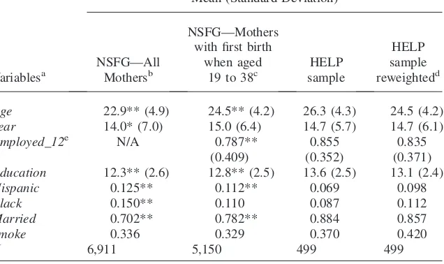
To explore whether labor supply effects of motherhood vary during the infant’s first year of life, Figure 1 presents employment rates of mothers in the HELP sample by months relative to when the child was born. Employment rates fall from around 85 percent before women become pregnant to 60 percent in the first four months after birth.11After that, employment increases slightly, reaching 66 percent 10 months af-ter birth. That employment does not vary significantly across the infant’s age in the first year supports the hypothesis that the estimated effects are not driven by the
Figure 1
Fraction of Mothers Employed and on Maternity Leave Relative to Month of Birth
10. Complete logit results are available from the author upon request.
actual age composition of babies at Month 21.12On the other hand, the fraction of mothers on maternity leave, shown in Figure 1, varies dramatically in the months surrounding birth (increases from close to 0 percent four months before birth to 52 percent in the birth month, falling significantly to only 4 percent five months later).13
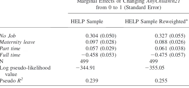
Women who have a child decide not only whether to have a job (the extensive margin) but also how many hours to work (the intensive margin). Unfortunately, the NSFG does not provide retrospective information on hours worked for women in the sample. Still, it provides information about whether a woman was working full time or part time and the availability of maternity leave. Using this information, work status is determined among four categories (full time, part time, maternity leave, and no job). Table 6 presents multinomial logit regression results for the im-pact on work status of having a first child. Having a child younger than one year old reduces the probability of working full time by 45.8 percentage points and it raises the probability of being in the other three categories. Interestingly, the increase in the probability of working part time is quite small (5.7 percentage points).
Table 6
Multinomial Logit Estimates. Impact of a First Child on Work Status
Marginal Effects of ChangingAnyChildren21
from 0 to 1 (Standard Error)
HELP Sample HELP Sample Reweighteda
No Job 0.304 (0.050) 0.327 (0.055)
Maternity leave 0.097 (0.028) 0.088 (0.026)
Part time 0.057 (0.029) 0.061 (0.038)
Full time 20.458 (0.053) 20.475 (0.057)
N 499 499
Log pseudo-likelihood value
2344.91 2355.05
PseudoR2 0.239 0.255
Note: Regression run on the HELP sample. The dependent variable has four categories: no job, maternity leave, part time, and full time. Covariates:Age0, Year0, Smoke0, Education0, Hispanic, Black, Married0, InsuranceCovered,andExperience0. NSFG: National Survey of Family Growth.
a. Observations are reweighted to match the age and year distribution in the sample of NSFG women whose first birth occurred when aged 19 to 38.
12. Reweighting the sample to have a uniform distribution of babies with respect to their ages in months yields a slightly smaller estimated effect of 24.3 percentage points.
VI. Robustness of the Empirical Strategy
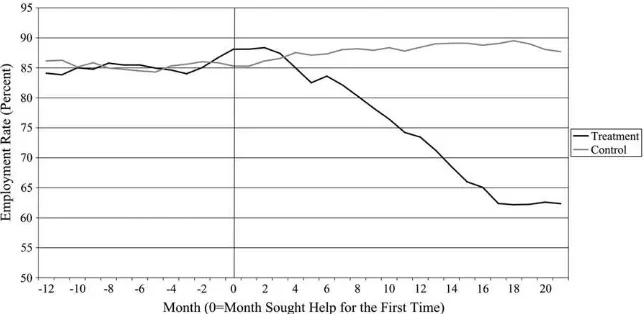
An important issue in the empirical strategy followed is whether the significant differences in employment between treatment and control women in Month 21 can be interpreted as the effect of treatment or as just heterogeneity in la-bor market attachment between groups. To analyze this issue, Figure 2 plots employ-ment rates of the treatemploy-ment and control groups for months –12 to 21. Employemploy-ment rates of both groups are quite similar for months –12 to 0, but they start diverging around Month 3 and are far apart by Month 21. The continuous decline in employ-ment rates for the treatemploy-ment group corresponds to the fact that as time goes by, ad-ditional women give birth until by Month 21 all had given birth.
Results from regressing employment status in Month 0 onAnyChildren21further reinforce the idea that differences in employment rates between the treatment and control group at Month 21 are not due to heterogeneity across these groups. The
t-value of the coefficient onAnyChildren21 is 0.80 in a specification with no cova-riates and 0.15 when all covacova-riates are added (the estimated coefficients are 0.028 and 0.006, respectively).14
Finally, a number of additional regressions are run to check whether the results are robust to changes in the specification. First, adding to the model with all covariates (presented in Column 4 of Table 5) an indicator for pregnancy in Month 21 margin-ally increases the estimated impact from 25.7 percentage points to 26.4. Second, replacing the main independent variableAnyChildren21with a variable that equals the total number of children born per woman by Month 21 slightly decreases the es-timate, to 24.7 percentage points. Finally, replacingAnyChildren21with two indica-tors for having one child or two children in Month 21 yields an estimated impact of
Figure 2
Employment Rates for Treatment and Control Groups
25.0 percentage points for the one-child indicator (and 46.4 for the two- children in-dicator).
VII. Comparison to Estimates from NSFG and
Census Data
This section compares estimates obtained using the HELP sample with estimates from similarly defined samples but without restricting them to women who sought help to become pregnant. As the HELP sample includes observations of fertility and labor supply for women at different points in time, its results should be compared to those from data sets with a similar distribution of observations across time (that is, from panel data or repeated cross-sections). I therefore compare esti-mates from the HELP sample to estiesti-mates from panel data from the NSFG (in Sub-section VIIA) and to estimates from census data for 1980 and 1990 (in VII.B).
A. Comparison to Estimates from NSFG Panel Data
I construct a panel data set from the NSFG Cycle 5 (the NSFG panel data) following requirements similar to those used to construct the HELP sample. The unit of obser-vation in this panel data is a woman-month. An obserobser-vation is included in the NSFG panel data if the woman was aged 21–40 in that month, was childless or had children younger than one year old, and was cohabitating or married.15
Because the HELP sample corresponds to a cross-section, to use the same source of variation when estimating both models, I construct a panel data set (the HELP panel data) including, for each individual in the HELP sample, observations for months –12 to 33 (remember that Month 0 corresponds to when the women first sought help with achieving pregnancy). Because the goal is to estimate the impact of having a child younger than one year old, monthly observations for a woman are dropped when her child is older than one year. Finally, for women who did not have a baby by Month 21, monthly observations of later months are dropped if they gave birth to a child.16
Table 7 presents summary statistics for the HELP panel data and the NSFG panel data. Mean values for key variables are similar and are only statistically significantly different for calendar year, children’s age in months, and proportion employed and with children. This last difference, the fraction of women with children, should be expected given that everyone in the HELP panel data did not have children for Month –12 up to (at least) Month 7.
Columns 1 and 3 of Table 8 present linear probability estimates of the impact of having a child younger than one year old on employment for women in the HELP and NSFG panel data sets, respectively. The key finding from comparing these
15. This age restriction is chosen because women in the HELP sample are aged 19–38 years old at Month 0 and then in Month 21 (when employment by fertility status is computed), almost all of them are 21–40 years old.
two columns is that the estimated impact for the NSFG panel data (0.259) is notably similar to the one obtained using the HELP panel data (0.260).
To gauge the robustness of the results, I estimate fixed-effects models using both panel data sets. Results are presented in Columns 2 and 4 of Table 8. For the HELP panel data, the estimated impact slightly decreases in absolute value to 0.234. In the case of the NSFG panel data, the estimated impact decreases in absolute value to 0.216. This result provides some evidence that women who have children tend to have lower employment rates in the months previous to become pregnant. Still, thet-value when testing the equality of the coefficients from fixed-effect models us-ing the two data sets is just –0.46.
Finally, I compare the estimated impact of having a child on work status (working full time, part time, maternity leave, and no job) for the two panel data sets. As Table 9 shows, estimates of the marginal effect of having a child on the probability of being in each of the four work-status categories are strikingly similar across the two data sets. The fact that estimates from the HELP panel data are so similar to those from the NSFG panel suggests that the endogeneity problem of fertility is not severe with
Table 7
HELP and NSFG Panel Data Descriptive Statistics
Mean (Standard Deviation)
Data NSFG—Cycle 5 (1995) NSFG—Cycle 5 (1995)
Sample HELP panel data NSFG panel data
Unit of observation Woman-month Woman-month
Employed 0.841* 0.808
AnyChildren 0.087** 0.171
Age 27.0 (4.4) 27.0 (4.4)
Education 14.0 (2.5) 14.0 (2.6)
Married 0.873 0.891
Smoke 0.361 0.327
Year(1970¼0) 14.8** (5.5) 15.6 (5.8)
Hispanic 0.059 0.066
Black 0.076 0.056
Baby age in months(for women with babies)
5.5** (3.5) 6.1 (3.7)
Number of observations 19,743 237,751
Number of women 467a 4,786
* Significantly different from the mean of the NSFG panel data at the 5 percent level. ** Significantly different from the mean of the NSFG panel data at the 1 percent level. Note: NSFG: National Survey of Family Growth.
Table 8
Impact of a First Child on Employment
Dependent Variable:EmployedCoefficient (Standard Error)
Data NSFG — Cycle 5 (1995) NSFG — Cycle 5 (1995)
Sample HELP panel data NSFG panel data
Unit of observation Woman-month Woman-month
Regression model OLS Fixed effects OLS Fixed effects
AnyChildren 20.260 (0.036) 20.234 (0.034) 20.259 (0.010) 20.216 (0.010)
Pregnant 20.092 (0.020) 20.065 (0.017) 20.074 (0.008) 20.050 (0.007)
Age 0.003 (0.004) 0.004 (0.007) 0.000 (0.002) 20.003 (0.003)
Education 0.011 (0.005) 0.032 (0.023) 0.005 (0.001) 0.029 (0.011)
Married 20.037 (0.033) 20.055 (0.025) 0.033 (0.011) 20.020 (0.010)
Smoke 20.026 (0.037) 0.091 (0.060) 0.016 (0.003) 0.007 (0.022)
Year(1970¼0) 0.008 (0.003) — 20.073 (0.019) —
Hispanic 20.103 (0.066) — 0.024 (0.018) —
Black 20.035 (0.048) — 20.020 (0.010) —
Constant 0.568 (0.143) 0.321 (0.287) 0.576 (0.045) 0.616 (0.158)
Adjusted R2 0.081 0.667 0.088 0.576
N 19,743 19,743 237,751 237,751
Note: Fixed-effects model for the HELP panel data includes dummy variables for individuals and months relative to the first time they sought help to become pregnant. Fixed-effects model for the NSFG panel data includes dummy variables for individuals and calendar years. Observations are clustered by individual. NSFG: National Survey of Family Growth.
The
Journal
of
Human
regard to its effects on biasing standard estimates of treatment effects. Another ex-planation is that endogeneity does create bias on estimates but the samples yield sim-ilar results because the differences in treatment effects across samples compensate for the bias (for example, there may an upwards bias in estimates on NSFG panel data, but the true treatment effect in the NSFG panel data is smaller than in the HELP panel data). This second explanation does not seem completely unlikely given that women in the HELP sample spent additional time and money to become pregnant.
B. Comparison to Estimates from 1980 and 1990 Census Data
In the HELP sample, fertility and other covariates are observed between 1972 and 1995. On average, those variables are observed in 1986, and the 10th and 90th per-centiles correspond to years 1978 and 1993, respectively. To construct samples com-parable to those from census data, women in the HELP sample are assigned to two new samples, the EARLY and LATE HELP samples, depending on whether they sought help to become pregnant before or after 1985.17
Using data from the 5 percent 1980 and 1990 Census Public Use Micro Samples (PUMS) I construct two samples (denoted as the 1980 and 1990 Census samples, re-spectively).18 The Census samples include married women aged 21–40, who are childless or have children younger than one year old. To capture women who are
Table 9
Multinomial Logit Estimates. Impact of a First Child on Work Status
Marginal effects of changingAnyChildren
from 0 to 1 (Standard Error)
Data NSFG — Cycle 5 (1995) NSFG — Cycle 5 (1995)
Sample HELP panel data NSFG panel data
Unit of observation Woman-month Woman-month
No Job 0.253 (0.038) 0.246 (0.009)
Maternity leave 0.115 (0.015) 0.116 (0.004)
Part time 0.010 (0.021) 0.005 (0.006)
Full time 20.378 (0.036) 20.368 (0.009)
N 19,743 237,751
Log pseudo-likelihood value
213,887.78 2195,128.98
PseudoR2 0.097 0.090
Note: The dependent variable has four categories: no job, maternity leave, part-time, and full-time. Cova-riates:Age, Year, Smoke, Education, Hispanic, Black, Married. Observations are clustered by individual. NSFG: National Survey of Family Growth.
‘‘at risk’’ of having a child and make the Census samples comparable to the HELP samples, only married women are kept in the Census and HELP samples.19
Table 10 presents descriptive statistics for the samples EARLY HELP, LATE HELP, 1980 Census, and 1990 Census. In the case of the HELP samples, the variable
Employedequals one if the woman had a job in Month 21. For the Census samples, it equals one if the woman had a job during the week previous to the survey. The var-iablesAnyChildren,Age,Education,HispanicandBlackare similarly defined in the four samples, and are all measured in Month 21 (for the HELP samples) or at the time of the survey (for the Census samples).
Summary statistics from Table 10 suggest that the 1980 and 1990 Census samples can be considered as reasonable comparison data sets for the EARLY and LATE HELP samples, respectively. Basic statistics on education and proportion black and Hispanic are remarkably close. Conversely, the proportion of women who have a child is significantly higher in the HELP samples. This finding should be expected, given that presumably all women in the HELP samples wanted to have children. Fi-nally, employment rates in the HELP samples, conditional on fertility status, are around 10 percent higher than in the Census samples (perhaps because employment is not defined exactly the same way in the NSFG as in the census).
Linear probability estimates of the impact of having a child younger than one year old on employment are presented in Table 11. Comparing Columns 1 and 2, we can see that the estimated effects are remarkably similar in the EARLY HELP sample and the 1980 Census sample (0.372 vs. 0.365). Similarly, the estimated impact is also quite close when comparing the LATE HELP sample and the 1990 Census sample (0.182 vs. 0.228). In both cases, the hypotheses of equality of the estimated coefficients cannot be rejected. From this set of results two important conclusions can be drawn. First, the esti-mated effects for the HELP sample for which I can identify an exogenous change in the fertility variable are nearly identical to the estimates obtained using OLS on comparable samples from census data, for which I do not control for the endogeneity of the fertility variable. They are also close to estimates obtained using panel data from the NSFG, as described in the previous subsection. Second, the results provide evidence of a significant reduction (about 40–50 percent) in the short-term impact of childbearing on female labor supply in the 1980–90 period.
VIII. Conclusions
This paper explores the issue of the causal effect of childbearing on female labor supply. This task is complicated by two factors. First, some researchers believe that women who have children at a certain age may have different baseline labor supply from women with similar observed characteristics who do not have chil-dren (Browning 1992). Second, the fertility decision may be endogenous to the woman and influenced by potential labor supply.
To deal with the problems of unobserved heterogeneity and endogeneity, I restrict my attention to a group of women who sought help to achieve pregnancy. In this sample, all
Mean (Standard Deviation)
Sample EARLY HELP 1980 Census LATE HELP 1990 Census
Sample description Married women in HELP sample who sought help before 1985
Married women aged 21 to 40 childless or with
children younger than 1 year old
Married women in HELP sample who sought help
on or after 1985
Married women aged 21 to 40 childless or with
children younger than 1 year old Time point 21 months after seeking
help for the first time
1980 21 months after seeking
help for the first time
1990
(1) (2) (3) (4)
Observation year 1981.5** (3.5) 1980.3 (0.0) 1991.0** (2.6) 1990.3 (0.0)
Employed 0.731 0.726 0.854* 0.796
AnyChildren 0.289** 0.158 0.358** 0.128
Age 26.1** (3.1) 27.2 (4.9) 30.2 ** (4.1) 29.3 (5.3)
Education 13.4 (2.4) 13.4 (2.6) 14.1 (2.6) 13.9 (2.5)
Hispanic 0.050 0.053 0.081 0.077
Black 0.065 0.061 0.069 0.061
N 216 287,292 224 301,371
* Significantly different from the mean of the comparable Census sample at the 5 percent level. ** Significantly different from the mean of the comparable Census sample at the 1 percent level. Note: The EARLY HELP sample is compared to 1980 Census data and LATE HELP to 1990 Census data.
Cristia
Table 11
Linear Probability Estimates. Impact of a First Child on Employment
Dependent variable:EmployedCoefficient (Standard Error)
Sample EARLY HELP 1980 Census LATE HELP 1990 Census
Sample description Married women in HELP sample who sought help before
1985
Married women aged 21 to 40 childless or with children younger
than 1 year old
Married women in HELP sample who sought help on or
after 1985
Married women aged 21 to 40 childless or with
children younger than 1 year old
Time point 21 months after seeking
help for the first time
1980 21 months after seeking help for the first time
1990
Mean of dependent variable 0.731 0.726 0.854 0.796
Independent variable (1) (2) (3) (4)
AnyChildren 20.372 (0.072) 20.365 (0.002) 20.182 (0.055) 20.228 (0.003)
Age 0.007 (0.012) 20.004 (0.000) 20.011 (0.007) 20.001 (0.000)
Education 0.024 (0.013) 0.030 (0.000) 0.021 (0.008) 0.031 (0.000)
Hispanic 0.042 (0.096) 20.047 (0.004) 20.259 (0.099) 20.087 (0.004)
Black 20.024 (0.109) 20.017 (0.003) 0.032 (0.062) 20.033 (0.004)
Year0 0.014 (0.011) — 20.002 (0.008) —
Constant 0.196 (0.270) 0.489 (0.006) 1.011 (0.272) 0.417 (0.007)
Adjusted R2 0.214 0.122 0.125 0.081
N 216 287,292 224 301,371
The
Journal
of
Human
the women wanted to have children, so the problem of endogeneity is minimized. More-over, because a major proportion of the fertility variable is random, results likely will not be contaminated by unobserved heterogeneity across groups. In fact, the attractive-ness of the strategy pursued here is that, by focusing on this sample of women, I mimic a hypothetical social experiment in which, for a group of women who want to have a child, some women are assigned children while others are not. Evidence favors the em-pirical strategy pursued: My results show that women’s employment, during months prior to seeking help becoming pregnant, is uncorrelated with subsequent fertility.
As shown in Section VII, this empirical strategy yields estimates similar to those from approaches that assume the exogeneity of fertility. At first, this finding seems to contradict the results of Angrist and Evans (1998) and Hotz, McElroy, and Sanders (2005) who reported significantly different OLS and IV estimates. A potential expla-nation for this divergence across studies is that the population of interest in them varies considerably. In this study, the parameter of interest applies to a female pop-ulation aged 19–38, mostly married and having children from planned pregnancies. For this population there is some evidence of small selection as women with and without children present similar demographic and economic observable characteris-tics in the constructed NSFG and census samples. Moreover, estimates from these samples are quite robust to the addition of different sets of covariates suggesting a small role for selection in the estimated effects.20
An interesting question that this paper leaves unanswered is why fertility and base-line employment seem to be uncorrelated. Many hypotheses may predict the opposite. For example, my strategy restricted the sample to women who are homogeneous in that all wanted to have a child at certain point in time, but clearly they could differ in how much they wanted to have a child, which in turn could be correlated with baseline labor force attachment.
A potential explanation for subsequent fertility being uncorrelated with baseline labor supply could be related to the fact that women in the HELP sample typically wait a num-ber of months before seeking help to achieve pregnancy. This ‘‘waiting’’ pattern could reduce the heterogeneity of women in the sample with respect to their baseline probabil-ity of having a child. Women with high probabilprobabil-ity of having a child achieve pregnancy right away and then do not seek help to become pregnant. Because individuals in the sample end up having similar probabilities of having a child, we approach the ideal sit-uation of random assignment, which is characterized as one in which all individuals have
equalprobability of being treated. If evidence is found suggesting that ‘‘waiting’’ is a suc-cessful empirical strategy in the sense that it increases the similarity between the treat-ment and control groups, then the same strategy could be applied to other evaluation problems in which dynamic assignment of individuals to treatment occurs.
References
Angrist, Joshua, and Williams Evans. 1998. ‘‘Children and their Parents’ Labor Supply: Evidence from Exogenous Variation in Family Size.’’American Economic Review 88(3):450–77.
Blau, Francine, and Adam Grossberg. 1992. ‘‘Maternal Labor Supply and Children’s Cognitive Development.’’Review of Economic and Statistics74(3):474–81. Bronars, Stephen, and Jeff Grogger. 1994. ‘‘The Economic Consequences of Unwed
Motherhood: Using Twin Births as a Natural Experiment.’’American Economic Review 84(5):1141–56.
Browning, Martin. 1992. ‘‘Children and Household Economic Behavior.’’Journal of Economic Literature30(3):1434–75.
Dunson, David, Donna Baird, and Bernardo Colombo. 2004. ‘‘Increased Infertility with Age in Men and Women.’’Obstetrics and Gynecology103(1):51–56.
Fuchs, Victor. 1989. ‘‘Women’s Quest for Economic Equality.’’Journal of Economic Perspectives3(1):25–41.
Goldin, Claudia. 1990.Understanding the Gender Gap.New York: Oxford University Press. Heckman, James, and V. Joseph Hotz. 1989. ‘‘Choosing among Alternative Nonexperimental Methods for Estimating the Impact of Social Programs: the Case of Manpower Training.’’ Journal of the American Statistical Association84(408):862–74.
Heckman, James, and Jeffrey Smith. 1995. ‘‘Assessing the Case for Social Experiments.’’ Journal of Economic Perspectives9(2):85–110.
Henshaw, Stanley. 1998. ‘‘Unintended Pregnancy in the United States.’’Family Planning Perspectives30(1):24–29.
Hotz, V. Joseph, Susan McElroy, and Seth Sanders. 2005. ‘‘Teenage Childbearing and its Life Cycle Consequences: Exploiting a Natural Experiment.’’Journal of Human Resources 40(3):683–715.
Jacobsen, Joyce, James Wishart Pearce III, and Joshua Rosenbloom. 1999. ‘‘The Effects of Childbearing on Married Women Labor Supply and Earnings: Using Twin Births as a Natural Experiment.’’Journal of Human Resources34(3):449–74.
Korenman, Sanders, and David Neumark. 1992. ‘‘Marriage, Motherhood, and Wages.’’ Journal of Human Resources27(2):233–55.
Miller, Amalia. 2005. ‘‘The Effect of Motherhood Timing on Career Path.’’ Department of Economics, University of Virginia. Unpublished.
Mosher, William. 1982. ‘‘Infertility Trends Among U.S. Couples: 1965–1976.’’Family Planning Perspectives14(1):22–27.
Rosenzweig, Mark, and Kenneth Wolpin. 1980. ‘‘Life-Cycle Labor Supply and Fertility: Causal Inferences from Households Models.’’Journal of Political Economy88(2):328–48. Ruggles, Steven, Matthew Sobek, Trent Alexander, Catherine A. Fitch, Ronald Goeken,
Patricia Kelly Hall, Miriam King, and Chad Ronnander. 2004. ‘‘Integrated Public Use Microdata Series: Version 3.0’’½Machine-readable database. Minneapolis, Minn.: Minnesota Population Center½producer and distributor.
Shapiro, David, and Frank Mott. 1994. ‘‘Long-Term Employment and Earnings of Women in Relation to Employment Behavior Surrounding the First Birth.’’Journal of Human Resources29(2):248–75.