HOUSEHOLD FOOD DEMAND IN INDONESIA:
A TWO-STAGE BUDGETING APPROACH
1Agus Widarjono
Universitas Islam Indonesia (widarjonoagus@gmail.com)
Sarastri Mumpuni Rucbha
Faculty of Economics, Universitas Islam Indonesia (mruchba@yahoo.com)
ABSTRACT
A two-stage budgeting approach was applied to analyze the food demand in urban areas separated by geographical areas and classified by income groups. The demographically augmented Quadratic Almost Ideal Demand System (QUAIDS) was employed to estimate the demand elasticity. Data from the National Social and Economic Survey of Households (SUSENAS) in 2011 were used. The demand system is a censored model because the data contains zero expenditures and is estimated by employing the consistent two-step estimation procedure to solve biased estimation.
The results show that price and income elasticities become less elastic from poor households to rich households. Demand by urban households in Java is more responsive to price but less responsive to income than urban households outside of Java. Simulation policies indicate that an increase in food prices would have more adverse impacts than a decrease in income levels. Poor families would suffer more than rich families from rising food prices and/or decreasing incomes. More importantly, urban households on Java are more vulnerable to an economic crisis, and would respond by reducing their food consumption. Economic policies to stabilize food prices are better than income policies, such as the cash transfer, to maintain the well-being of the population in Indonesia
Keywords: Urban, Two-Stage Budgeting, QUAIDS, Price and Income elasticity
INTRODUCTION
The high1economic growth during the period from 1970 to 1994 caused Indonesia to be reclassified from a low income category country to a middle income category country. The GDP per capita was $1,124 in 1996. It dropped drastically to only $459 in 1998 because of the economic crisis. However, after the economic recovery, Indonesia’s economy has moved towards that of a middle income country. GDP per capita increased to $1,859 in 2007 and rose to $3,495 in 2011 (World Bank, 2012). As the fourth most populous country in the world, Indonesia has been experiencing rapid urban growth since the mid-1980s. The urban popu-lation was only 22.4 percent in 1980, but had
1
This research was fully funded by DIKTI through a Fundamental Research Grant for the year 2014-2015
grown to 35.91 percent in 1995. The proportion of people living in urban areas had increased to 48 percent by 2005 and it has been more than 50 percent of the total population since 2006 (at 50.31 percent). The urban population is predicted to reach 60 percent by 2025 (Central Bureau of Statistics, 2011).
transfor-mation, the Gini coefficient only fluctuated marginally with the range being from 0.32 to 0.37 during the 1964-2007. The Gini coefficient was relatively stable during the next two consecutive years (2008 and 2009) by 0.37, but it increased to 0.38 and the 0.41 in 2010 and 2014 respectively (Central Bureau of Statistics, 2015). The stability of the income distribution can also be illustrated by the share of the top 20 percent to the bottom 40 percent of consumer household expenditures. This ratio barely moved from 2.33 in 1964 to 2.08 in 2005 (Mishra, 2007). However, the ratio has increased in recent years. It was 2.86 in 2012 and became 2.91 in 2014 (Central Bureau of Statistics, 2014). The Gini coefficient for urban areas was close to the national average. It was 0.34 in 1964, but increased to 0.36 in 1998 because of the economic crisis, and then decreased to 0.32 in 2005 (Mishra, 2007). However, the Gini coefficient for urban areas recently increased. It was 0.37 during 2007 to 2009 but rose to 0.38 and 0.43 in 2010 and 2014 respectively (Central Bureau of Statistics, 2015). In fact, the national Gini coefficient is primarily influenced by the urban Gini coefficient, because Indonesia’s urban population has increased rapidly over the last four decades.
Economic growth and urbanization have contributed not only to an increase in incomes, but also to drastic changes in the composition of the food demand in Indonesia. The higher incomes contribute to a greater demand for more expensive sources of calories such as meat, fruit, vegetables, and processed food products. The proportion of total calories derived from low-value sources of calories, such as starchy roots, has declined, while the proportion of total calories derived from high values foods such as meat, fish/sea food, fruit, vegetables and vegetable oil has increased during the 1961-2003 period (Rada & Regmi, 2010).
The monthly average budget share of cereals and tubers to the total food expenditure was 17.56 percent in 1999 but it dropped slightly to 12.88 percent in 2013. Monthly expenditure for fish, meat, eggs and milk, vegetables, fruit and oil and fats, as high value foods, to the total food expenditure were 22.12 percent in 1999 and increased steadily to 37.24 percent in 2014.
Regarding this income growth, the rapid urbanization and changes in consumption from low-value to high-value foods, it is important to estimate the demand for food in Indonesia. This study has several goals. The firstly, the purpose of this study is to estimate the demand for food from ten food groups encompassing cereals, fish, meat, eggs and milk, vegetables, fruit, oil and fats, prepared foods and drink, other foods and tobacco products in Indonesia. Secondly, because of differences in the income distribution and consumption patterns of households, it is also important to estimate the demand for food in separate areas, both in Java and outside Java, based on the income level. Thirdl, this study applies the new demand system model. Unlike most previous studies on food demand in Indonesia which used the LA/AIDS with a linear price index in the model except for Fabiosa et al., (2005) who used a LinQuad model and Pangribowo and Tsegai (2011) and Fahar et al., (2013) who used the QUAIDS model, this study uses QUAIDS but employs a non-linear price
The rest of this paper is as follows. The food consumption pattern in urban Indonesia is highlighted in Section II. The next section presents the model’s specifications, estimation procedures and data. Section IV discusses the findings of this study, including the simulation policy. The final section of this study discusses the conclusions and possible implications for policies regarding these results.
FOOD CONSUMPTION PATTERNS IN INDONESIA
Food expenditure was relatively high com-pared to non-food expenditure in 1990, at 60.36 and 39.64 percent respectively. However, food expenditure tended to decrease overtime and non-food expenditure increased during the
1990-2005 period. Non-food expenditure has exceed-ed food expenditure since 2011. The percentage for food expenditure generally decreased as the purchasing power of consumers increased. This indicated that food consumption in Indonesia followed the pattern of Engel’s law.
Food expenditure has fluctuated over the period from 1999 to 2013. Food expenditure was 55.3 percent of total expenditure in 1996 and rose
sharply
to 62.9percent in 1999 due to the impact of the economic crisis in 1997.
However,food
expenditure again decreased to 50.62 percent by 2009, increased slightly to 51.43 percent in 2010and decreased slightly to
50.66 percent in 2013 (
Central Bureau of Statistics, various issues).
On average, the total specific food expenditure to total expenditure varied over the 1999-2013 period. Cereals were dominant in the total food expenditure at the beginning of that period, but the percentage expenditures decreased. Meanwhile, prepared food and beverages have been steadily increasing and recently replaced cereals as the dominant food expenditure. Therefore, prepared food and beverages now dominate total food expenditure, followed by cereals, tobacco and betel, fish, vegetables, and eggs and milk. The expenditure on tobacco and betel also contributed a relatively high figure toward the monthly average per capita expenditure in Indonesia. The lowest food expenditure was for tubers, which account for less than 1% of total expenditure. This is not surprising as tubers, which include such items cassava and sago, are a low-value staple food in the Indonesian diet.Figure 1. Percentage of Low and High-Value Food Expenditure to Food Expenditure, Indonesia, 2000-2013
Note: Low-value foods consist of cereals and tubers, high-value foods consist of fish, meat, eggs and milk, vegetables, legumes, fruit, and oil and fats, other foods consist of beverages, spices, miscellaneous food items, prepared food and beverages, and tobacco consists of tobacco and betel.
Source: Statistical Yearbook of Indonesia, Central Bureau of Statistics, various issues
MODEL SPECIFICATION AND DATA 1. Model Specification and Estimation
Procedures
This study investigates the food demand in Indonesia for ten food groups. However, a full demand system for these ten food groups needs to estimate a large number of parameters. Therefore, this study uses a two-stage budgeting approach in order to reduce the number of parameters to be estimated. In the first-stage budgeting, the total expenditure is allocated between food and non-food commodities. Food expenditure is then allocated between the ten food groups in the second-stage budgeting.
Weak separability is important for multiple stage budgeting in demand system’s analysis. If food is assumed to be weakly separable from non-food, then the consumers’ utility maximization decision can be decomposed into several budget stages procedures (Deaton & Muellbauer, 1980). Because this study applies the two-stage budgeting procedure, in the first- stage budgeting, the study estimates the demand for food and non-food items. Then, it estimates
the demand for each of the ten food groups in the second-stage budgeting.
There are two broad groups of goods for the first stage of the demand system namely food and non-food items. The functional form for the first-stage demand system is from Working (1943)-Lesser (1963) to estimate the demand elasticity for food as:
�" = �%+ �"��� + ,+-.�"+����+
�"2 ,
2-. ��+ �" (1)
where � and � are commodities, �" is the share of total expenditure allocated to the �th commodity,
�+ is the price of the �th commodity, � is the household’s expenditure on commodities, �2 is
the demographic variable consisting of the household’s size, the educational level of the head of the household (years of schooling), the age of the household’s head, the gender of the household’s head, and two quarter dummy variables (quarter 2 and 3).
The uncompensated (Marshallian) price
(∈"+) and expenditure elasticities (∈") can be derived from equation (1) as follows:
0.00 5.00 10.00 15.00 20.00 25.00 30.00 35.00 40.00 45.00
2000 2001 2002 2003 2004 2005 2006 2007 2008 2009 2010 2011 2012 2013
∈��=�����−δ�� (2)
∈"= 1 + . @A
[ �"] (3)
δ�� is the Kronecker Delta. If �≠� then it is zero and unity otherwise. The own-price, cross-price and expenditure elasticities are evaluated at sample means. This study uses Engle’s function to estimate income elasticity because the Working-Lesser model does not provide a direct estimate of it as follows:
��� = �%+ �.��� + ∅��� +
�"2 ,
2-. ��+ �" (4)
where � is the household’s expenditure on food,
� is the total expenditure on food and non-food items, � is the price index of food, and �� are the demographic variables that are the same as previously defined in equation (1). Following Chern et al., (2003), the income elasticity is estimated as:
∈L=∈" �. (5)
For the second-stage demand system, the Quadratic Almost Ideal Demand System (QUAIDS) developed by Banks et al., (1997) is used. The QUAIDS has the properties of both a flexible functional form and a non-linear Engel 1980). We did incorporate demographic variables into the intercept in equation (6). These demographic variables are the same as those in
the Working-Leser model. The expenditure variables in equation (6) are endogenous variables. To solve the endogeneity problem, this study follows the procedures proposed by Blundell and Robin (1999) using instrumental variables. The properties of the neoclassical demand theory consisting of adding-up, homogeneity and Slustky’s symmetry can be dependent variables are the limited dependent variables or the censored model in the demand system, and cause biased estimation. This study employs the consistent two-step estimation procedure for a system of equations with limited dependent variables (Shonkwiler & Yen, 1999). The first step is to estimate a probit regression to determine the probability of buying a given type of food. The probit regression for food demand and the demographic variables previously defined in the Working-Lesser model.
The next step included the cumulative distribution function and the probability distribution function in the QUAIDS. Therefore, the QUAIDS model used in this study was (Shonkwiler & Yen 1999):
��={��+�=1��������+�������+��(�
��)2+��}Φ.+���(.)+�� (9)
(CDF) and Probability Distribution Function (PDF), respectively.
In a conventional model without censoring, the adding-up condition holds in the right-hand side of system equation (9). However, with a censoring model, the right-hand side of system equation (9) does not add up to unity across all the equations of the demand system and the adding-up condition does not hold. As a result, the second step estimation of the system equation in the demand system should be estimated on the entire � equations (Yen et al., 2002).
The Marshallian price elasticity of the QUAIDS model is calculated as follows:
���=1�����−(��+2λ��������)��ℎ+�=1
��������−λ�����(�����)2Φ� −δ��
...(10)
The expenditure elasticity of the QUAIDS model can be calculated as:
��=1+1��[ ��+2�������]� (11)
� is the Kronecker delta (1 if �=� and 0 otherwise).
Because this study applies the second stages budgeting, the demand elasticities in the second-stage budgeting are conditional on total food expenditures in the first-stage budgeting. Following Edgerton (1997), unconditional price (�"+) and expenditures (�") elasticities are calculated as:
�"+= �"++ �"[�++∈"+ �+] (10)
�" = �" ∈" (11)
where �"+ is the conditional price elasticity, �" is the conditional expenditure elasticity for �th food groups in the second-stage budgeting, ∈"+ is the price elasticity of food in the first-stage budgeting, �+ is the expenditure share of �th
food groups, and ∈" is the unconditional
expenditure elasticity for food in the first-stage budgeting.
Finally, economists are concerned about income elasticity instead of expenditure
elasticity, being the main economic policy. The income elasticity of food for the �th commodity is given by (Park et al., 1996; Zheng & Henneberry, 2010):
Ω" = �" ∈L (12)
where Ω" is the unconditional expenditure
elasti-city for the �th commodity within the food groups in the second-stage budgeting, and ∈Lthe
income elasticity of food in the first-stage budgeting.
The last step in this study is to use the calculated demand elasticity to estimate the expected changes in demand for the food groups being studied. It is a fact that the food consumed is affected by changes in a particular food’s price and/- or the per capita food expenditure through the interdependent demand relationship. The relative changes in food demand are associated with the relative changes in food prices and income, and can be formulated as (Shan, 1988; Zheng & Henneberry, 2012):
ln��=����∆ln��+η�∆ln� (13)
where∆ ln �2 = ∆�2/�2is the percentage change
in food demand of food group k, ∆ ln �+= ∆�+/�+represents the percentage change in the price of food group j and ∆ ln � = ∆�/� denotes the percentage change in household income.
2. Data
Statistics (CBS), 40 percent of the lowest expenditure households were classified as low income (poor households), 40 percent of those with a medium household expenditure were considered to be middle income (medium households) and 20 percent with the highest household expenditure were classed as high income (rich households).
This study used SUSENAS 2011 and consisted of 215 food commodities. The CBS classifies food consumption into 14 food groups. For the purpose of this study, we regrouped the 14 groups to form our 10 food groups, according to their similar nutritional components. The 10 food groups consisted of: (1) Cereals encom-passing cereals and tubers; (2) fish; (3) meat; (4) eggs and milk; (5) vegetables; (6) fruit; (7) oil and fats encompassing oils and fats and legumes; (8) prepared food and drinks encompassing beverages and prepared food; (9) other foods encompassing spices and miscellaneous foods; and (10) tobacco products. Non-food expen-diture consisted of 6 commodity groups encompassing housing and household facilities; goods and services; clothing, footwear and headgear; durable goods; taxes and insurance; and parties and ceremonies.
The SUSENAS provided information on prices for each food commodity. The weighted average of prices within groups using the budget share as a weight was used to calculate the aggregate price for each food group (Moschini, 1995). If missing or unreported aggregate prices existed, these prices were calculated by regressing the observed prices on regional dummies, seasonal dummies, and income (Jensen & Manrique, 1998). Total household expenditure was used as a proxy for income (Deaton, 1996; Moeis, 2003).
In the first-stage budgeting, this study estimated the demand for food and non-food items. Monthly food and non-food expenditure data were used to estimate the food and non-food spending in the first-stage budgeting. However, the SUSENAS does not provide information about prices for non-food expenditure. Following the study of Jensen and Manrique (1998), this study used the consumer
price index for non-food items. The aggregate price for the non-food commodity group was calculated using an average of the consumer price index for non-food items in each province. If a province had more than one city, the aggregate price for the non-food items in each province was calculated as the average price for those cities.
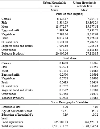
Table 1 describes the summary statistics for urban households both in Java and outside Java. The most expensive food is meat and the least expensive is prepared food for both urban Java and the other islands, but on average the prices for all the food groups are more expensive on Java than on the other islands. The largest share of the budget is spent on prepared food and drinks, both in urban areas on Java and outside Java, then comes cereals. These statistics indicate that urban households consume mostly “fast foods” and the budget share for cereals, including rice, is relatively high because rice is a staple food in Indonesia. Food expenditure in urban areas outside Java are higher than those in urban areas on Java.
RESULTS AND DISCUSSION 1. Demand Elasticity
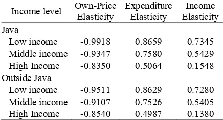
The Working –Leser model for the first-stage budgeting, consisting of food and non-food commodity groups, was estimated using the Ordinary Least Squares (OLS) method. Food demand in the first-step demand system was run separately for the different income groups for both urban areas in and outside Java. Then, the price and expenditure elasticity for food was calculated from the estimated parameter of the Working-Leser model using equations (2) and (3). Finally, the expenditure elasticity obtained from the Working-Leser model and Engle’s function could be used to derive income elasticity by applying equation (5)2. The first-step demand system provides an unconditional price and expenditure elasticity for food in the first-stage budgeting.
2
The price, expenditure and income elasti-cities of the ten food groups in the first-step demand system across the income levels for both urban areas on and outside Java are represented in Table 2. The price, expenditure and income elasticities vary according to income levels in both areas. As expected, all the own-price elasticities for food are negative and inelastic across income levels in the urban areas in and outside Java. Poor households in all urban areas are more responsive to prices than rich households. However, own-price elasticities in the urban areas of Java are higher than those in urban areas on other islands, across all income levels. All food expenditure and income elasticities are positive but inelastic. Like price
elasticitiy, expenditure and income elasticities become more inelastic moving from poor households to rich households in both sets of urban areas.
The demand system in the second-stage budgeting consisted of food groups encom-passing cereals, fish, meat, eggs and milk, vegetables, fruit, oil and fats, prepared food and drinks, other foods and tobacco products. SUSENAS’s 2011 results provided some zero expenditure for a given food type from its survey of urban areas.
Table 2. Price, Expenditure and Income Elasti-cities of Food Demand by Income Groups,the First-Stage Demand, Urban Indonesia, 2011
Table 1. Summary Statistics, Urban Households, Indonesia, 2011
Urban Households in Java
Urban Households outside Java
Mean Mean
Price of food (rupiah)
Cereals 6,124.87 7,054.77
Fish 8,384.03 13,895.24
Meat 13,972.57 15,577.58
Eggs and milk 1,991.54 2,932.75
Vegetables 7,398.76 8,657.63
Fruit 8,039.84 9,476.24
Oils and Fats 2,521.88 2,984.58 Prepared food and drinks 1,092.66 1,255.36 Other foods 7,018.25 8,151.63 Tobacco Products 20,409.06 27,180.85
Food share
Cereals 0.1608 0.1665
Fish 0.0524 0.1250
Meat 0.0383 0.0364
Eggs and milk 0.0590 0.0598
Vegetables 0.0758 0.0902
Fruit 0.0413 0.0454
Oils and Fats 0.0757 0.0582
Prepared food and drinks 0.3582 0.2703
Other foods 0.0458 0.0419
Tobacco Products 0.0928 0.1064 Socio Demographic Variables
Household size 3.70 4.08
Age of household’s head 47.51 45.17 Education of household’s
head
9.19 10.12
Food expenditure 265,705.03 346,623.11 Total expenditure 2,571,513.57 3,140,359.54
Income level Own-Price Middle income -0.9347 0.7580 0.5429 High Income -0.8350 0.5064 0.1548 Outside Java
Low income -0.9511 0.8629 0.7280 Middle income -0.9107 0.7526 0.5405 High Income -0.8540 0.4987 0.1380 Source: Estimated using the 2011 SUSENAS
The zero expenditure for cereals, fish, meat, eggs and milk, vegetables, fruit, oil and fats, prepared foods and drinks, other foods and tobacco products were 4.35 percent, 15.54 percent, 51.60 percent, 14.62 percent, 7.86 percent, 23.25 percent, 6.57 percent, 0.21 percent, 4.45 percent, and 37.36 percent respectively. In order to avoid any bias estimated parameters because of a zero observation in the demand system, the consistent two-step estimation procedure was employed. In the first-step estimation, the probit model was applied to estimate the studied food groups separately, using the maximum likelihood to calculate the CDF and PDF. In the second-step estimation, the food demand for the ten food groups was estimated by including the CDF and PDF into the QUAIDS, using a Full Information Maximum Likelihood estimation (FIML) with the imposition of homogeneity and symmetry conditions.
The AIDS assumes that Engel’s curve is linear for income but the QUAIDS allows for a quadratic term in the estimation of this curve. Among the 60 estimated values of the quadratic Engle curve, 59 coefficients were statistically significant at the 10 percent or lower levels. These results indicated that the QUAIDS model was appropriate, and a superior model to the AIDS model in estimating the food demand system in Indonesia across income levels.3
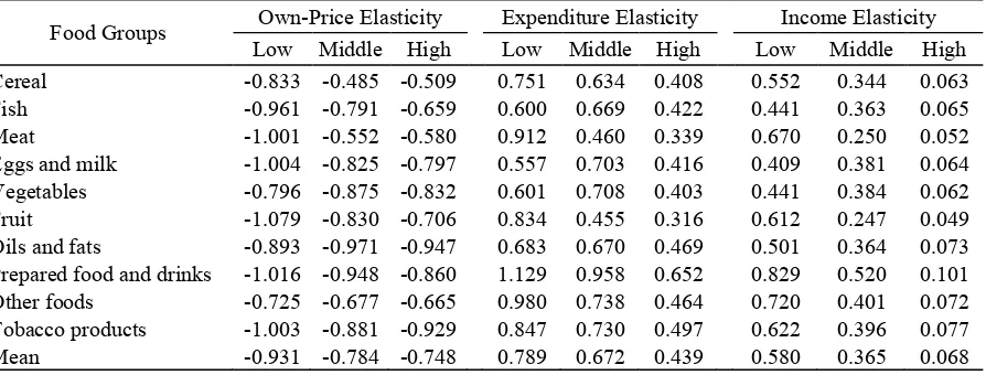
Table 3 and 4 report the conditional price and expenditure elasticities for the ten food groups studied, across income levels both in urban areas in and outside Java4. All own-price elasticities are negative across the income strata
3
The estimations and results in the second-stage budgeting are available upon request
4
The cross-price elasticities are not reported to conserve space and are available upon request
and the results are consistent with the economic theory. As expected, poor households in urban areas in and outside Java are more responsive to price changes. All conditional expenditure elasticities are positive across the income strata. Like own-price elasticities, rich households are less responsive to expenditure changes than poor households.
According to the two-stage budgeting approach in estimating demand elasticity, the price and expenditure elasticities for the studied food groups in the second-stage budgeting were conditional upon both the price and expenditure elasticities in the first-stage budgeting. There-fore, the demand elasticities in this study were unconditional demand elasticities, and were calculated using equations (10), (11) and (12).
Table 3. Conditional Own-Price and Expenditure Elasticity by Income Groups, The Second-Stage Demand, Urban Java, Indonesia, 2011
Food Group Own-Price Elasticity Expenditure Elasticity Low Middle High Low Middle High Cereal -0.8341 -0.4928 -0.5221 0.8679 0.8358 0.8057 Fish -0.9616 -0.7942 -0.6677 0.6930 0.8820 0.8325 Meat -1.0012 -0.5541 -0.5866 1.0531 0.6067 0.6686 Eggs and milk -1.0042 -0.8290 -0.8088 0.6432 0.9271 0.8216 Vegetables -0.7960 -0.8790 -0.8395 0.6940 0.9338 0.7952 Fruit -1.0795 -0.8314 -0.7122 0.9630 0.6007 0.6248 Oils and fats -0.8933 -0.9752 -0.9548 0.7883 0.8841 0.9269 Prepared food and drinks -1.0199 -0.9783 -0.9449 1.3043 1.2634 1.2872 Other foods -0.7255 -0.6798 -0.6703 1.1316 0.9734 0.9168 Tobacco Products -1.0035 -0.8877 -0.9422 0.9784 0.9634 0.9819 Source: Estimated using the 2011 SUSENAS
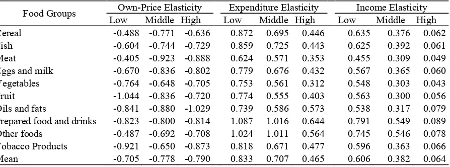
Table 4. Conditional Own-Price and Expenditure Elasticity by Income Groups, The Second-Stage Demand, Urban Off Java, Indonesia, 2011
Food groups Own-Price Elasticity Expenditure Elasticity Low Middle High Low Middle High Cereal -0.4979 -0.7834 -0.6511 1.0104 0.9239 0.8939 Fish -0.6106 -0.7550 -0.7455 0.9952 0.9629 0.8889 Meat -0.4057 -0.9261 -0.8945 0.7237 0.7586 0.7076 Eggs and milk -0.6724 -0.8414 -0.8128 0.9028 0.8979 0.8654 Vegetables -0.7688 -0.6539 -0.7145 0.8726 0.7451 0.6254 Fruit -1.0452 -0.8394 -0.7260 0.8965 0.7376 0.8087 Oils and fats -0.8442 -0.8841 -1.0360 0.8568 0.7783 1.1482 Prepared food and drinks -0.8383 -0.8326 -0.8809 1.2599 1.3501 1.2919 Other foods -0.4900 -0.6965 -0.7133 1.1862 1.3434 1.1310 Tobacco Products -0.9258 -0.6587 -0.8884 0.9482 0.8919 0.9568
Source: Estimated using the 2011 SUSENAS
Table 5. Unconditional Own-Price and Expenditure Elasticity by Income Groups, The Second-Stage Demand, Urban Java, Indonesia, 2011
With the exception of prepared food and drinks for low income households, all the unconditional expenditure elasticities are positive but inelastic. However, the main concern of economic policies is income elasticity instead of expenditure elasticity. All income elasticities are positive but inelastic (necessity goods) and relatively stable across the income levels. Prepared food and drinks are the most responsive to income changes for all income levels. The income elasticity of the cereal group, as a staple food, is relatively low compared to other food groups across the income strata. Most of the high value foods such as fish, meat, eggs and milk, vegetables, fruit, and oil and fats are less sensitive to income changes across income levels compared to the other food groups. Broadly speaking, income elasticity becomes more elastic as it moves towards the lower income households.
Unconditional demand elasticities for the urban areas outside Java are shown in Table 6. Like urban areas in Java, all the own-price elasticities are negative and inelastic with the exception of fruit and oils and fats for the low and high income groups respectively. Higher income households are less responsive to price changes than the lower income households. Cereals, as a staple food, are less responsive to price changes for low income households, but become more responsive to price changes when moving towards higher income households. Meat is inelastic for poor households but it is elastic for higher income households. The
demand for rice for urban families outside Java is less responsive to price changes compared to urban families in Java. Estimated own-price elasticities for high-value foods such as fish, eggs and milk, vegetables, fruit, and oil and fats in urban areas outside Java are less sensitive to price changes compared to urban areas on Java across all income levels. In general, urban households outside Java generally show less own-price elasticity than urban households on Java.
All food groups have income elasticities which are smaller than unity (necessity goods). Like Jansen and Manrique (1998), income elasticity becomes more elastic as it moves toward the lower income households. Prepared food and drinks are the most responsive to income changes for all income levels. The income elasticity of the cereal group is more elastic moving from higher to lower income households. More importantly, the demand for cereals in urban areas outside Java is more responsive to income changes than those urban areas in Java. Fish, meat, eggs and milk, vegetables, fruit, and oil and fats, as high value foods, mostly have income elasticities which are smaller than those of the other food groups. However, the income elasticities of those high value foods for urban areas outside Java are generally higher than for the urban areas on Java. In general, urban households outside Java are more responsive to income changes than urban households on Java.
Table 6. Unconditional Own-Price and Expenditure Elasticity by Income Groups, The Second-Stage Demand, Urban Outside Java, Indonesia, 2011
2. Policy Simulation
The estimated price and income elasticities were then used to analyze the impact of changes in prices and income on tahe demand for food. This study used equation (13) to the estimate the change in demand for the studied food groups across income levels. Three scenarios were considered for simulating the effect of price and income changes on demand for the studied foods. Scenario 1 considered an increase of 10 percent in the price of all the studied food groups, while holding incomes constant. Scenario 2 considered a decrease in income of 10 percent , assuming the price of food did not
change. The last scenario involved increasing the price of all the studied food groups by 10 percent and decreasing incomes by 10 percent simultaneously. The last scenario represents an economic crisis, marked by falling incomes and the rising price of goods. The simulation was expected to give information on who would be most affected by the increase or decrease in prices and incomes. The results of this simulation are expected to provide important information about formulating food policies and welfare analysis to government. The simulation results are reported in Tables 7 and 8.
Table 7. Effect of change in price and income on food demand, Urban Java, 2011
Scenario 1 Scenario 2 Scenario 3 Low Middle High Low Middle High Low Middle High
Cereals -0.084 -0.046 -0.058 -0.055 -0.034 -0.006 -0.140 -0.080 -0.065 Fish -0.056 -0.076 -0.065 -0.044 -0.036 -0.007 -0.101 -0.112 -0.072 Meat -0.104 -0.023 -0.040 -0.067 -0.025 -0.005 -0.171 -0.048 -0.045 Eggs and milk -0.045 -0.078 -0.064 -0.041 -0.038 -0.006 -0.086 -0.116 -0.070 Vegetables -0.038 -0.086 -0.052 -0.044 -0.038 -0.006 -0.082 -0.125 -0.059 Fruit -0.095 -0.006 -0.029 -0.061 -0.025 -0.005 -0.157 -0.031 -0.034 Oils and fats -0.080 -0.079 -0.067 -0.050 -0.036 -0.007 -0.130 -0.115 -0.075 Prepared food and drinks -0.089 -0.092 -0.069 -0.083 -0.052 -0.010 -0.172 -0.144 -0.079 Other foods -0.082 -0.072 -0.074 -0.072 -0.040 -0.007 -0.153 -0.112 -0.081 Tobacco Products -0.097 -0.088 -0.081 -0.062 -0.040 -0.008 -0.159 -0.127 -0.089
Source: Estimated using the 2011 SUSENAS
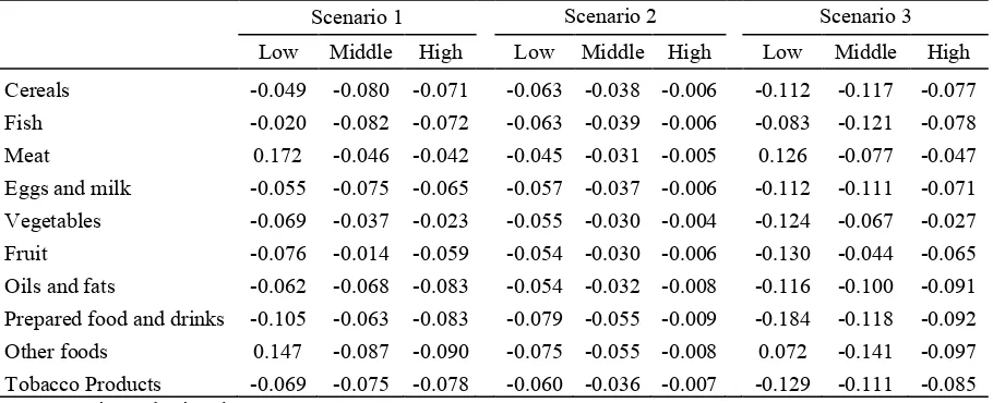
Table 8. Effect of change in price and income on food demand, Urban Off Java, 2011
Scenario 1 Scenario 2 Scenario 3 Low Middle High Low Middle High Low Middle High
The simulation resulted in some important findings. Firstly, price changes while holding incomes unchanged (scenario 1) would have an areas. However, urban households outside Java had a more adverse impact on the demand for food than those urban households on Java. Secondly, decreasing incomes by 10 percent (scenario 2) would reduce the demand for the studied food groups across all income groups. Like scenario 1, the wealthier families suffer less than the poor families and urban households outside Java would reduce their consumption of food as income decrease more than the urban households on Java would. Thirdly, increasing the price of food and decreasing incomes simultaneously had the biggest negative impact on food demand in both urban areas, compared to the other scenarios. In general, the third scenario had more of an adverse impact on the urban areas in Java compared to those on other island. Therefore, it can be concluded that if an economic crisis hit Indonesia, the urban families on Java would suffer more than the urban families on outside Java. Fourthly, an increase in the price of food had more of a negative impact on the demand for food than a decrease in income had.
CONCLUSIONS AND RECOMMENDATIONS
This study estimated the demand for food using the two-stage budget procedures with weak separability. The complete demand system of urban households for the ten food types studied was estimated using the Quadratic Almost Ideal Demand System (QUAIDS). The National Social and Economic Survey of Household in Indonesia (SUSENAS) in 2011 was used to accomplish this study. Because diets differ across geographical areas, this study separated the food demand into urban areas on Java and outside Java.
The findings indicated that the estimated price and income elasticities for all income groups looked quite reasonable and varied slightly for different income levels. The own-price elasticities of demand became less elastic when moving from low to high income house-holds. Urban households on Java were more responsive to price changes than those urban households outside Java. As expected based on income elasticities, all the food groups studied were necessity goods. The income elasticities of demand also showed as being less elastic from low to high income families. However, urban households outside Java were more responsive to changes in income compared to urban households in Java. Most of the high value foods were not responsive to income changes. Urban households outside Java were more responsive to the demand for cereals, as a staple food, people in the East Nusa Tenggara Area.
Our simulations showed that an increase in food price had bigger and worse impact than a decrease in household incomes. As food prices increase, poor households suffer more than wealthier households. These findings imply that economic policies to stabilize food prices are more suitable than an income policy, such as cash transfers, in maintaining the welfare of households. However, poor families may also benefit from an income policy. Therefore, an income policy, such as the cash transfer one, would also help poor families to maintain their welfare. The simulation also indicates that urban households on Java are more vulnerable to an economic crisis than urban households outside Java associated with their food consumption. The results imply that urban families on Java have higher risk of nutritional deficiencies than urban families on other island.
are different across all the islands outside Java. Future research should investigate the demand for food on each separate island, such as Sumatra, Kalimantan, Sulawesi and Papua. It is also important to analyze the food demand for rural households, because food consumption patterns are definitely different for urban and rural households. This study used data from 2011, future research needs to use the latest available data due to ongoing rapid urbanization process taking place in all the regions of
Economics and Statistics 76 : 351-56
Banks, J., R. Blundell, and A. Lewbel. 1997. “Quadratic Engle Curves and Consumer Demand.” The Review of Economics and
Statistics 79:527-539.
Blundell, R., and J.M. Robin. 1999. “Estimation in Large and Disaggregated Demand Systems: An Estimator for Conditionally Linear Systems.” Journal of Applied
Econometrics 14:209-232.
Central Bureau of Statistics (CBS).Statistical
Yearbook of Indonesia, various issues.
Chern, S. Wen, K. Ishboshi, K. Taniguchi and Y. Tokoyama. 2003. Analysis of Food Consumption Behavior by Japanese House-holds. Food and Agricultural Organization: Economic and Social Development, Paper 152.
Deaton, Angus and J. Muellbauer. 1980. “An Almost Ideal Demand System.” American
Economic Review 70: 312-326.
Deaton, Angus. 1996. The Analysis of House-hold Surveys: A Microeconometric
Ap-proach to Development Policy. Baltimore:
John Hopkins University Press
Edgerton L. David. 1997. "Weak Separability and the Estimation of Elasticities in Multistage Demand System." American
Journal of Agricultural Economics 79:
62-79.
Fabiosa, J.F., Jensen, H., and Yan, D. 2005. “Household Welfare Cost of the Indonesian Macroeconomic Crisis”. Selected Paper prepared for presentation at the American Agricultural Economic Association Annual Meeting, Rhode Island, 24-27 July. http:// katan Quadratic Almost Ideal Demand System. http://www.researchgate.net/ publication/280976063. (Accessed May 31st, 2016)
Jensen, Helen H., and Justo Manrique. 1998. “Demand for Food Commodities by Income Groups in Indonesia.” Applied Economics 30: 491-501.
Leser, C.E. 1963. "Forms of Engle Functions."
Econometrica 31: 694-763.
Mishra, S., Candra. 2007. “Economic Inequality in Indonesia: Trends, Causes and Policy Response.” http://www.strategic-asia.com/ indonesia/reports.html. Accessed February 24th, 2014.
Moeis, J. Prananta. 2003. “Indonesian Food Demand System: An Analysis of the Impact of the Economic Crisis on Household Consumption and Nutritional Intake.” Unpublished Doctor of Philosophy’s Dissertation.The Faculty of Columbian College of Art and Sciences, George Washington University.
Moschini, G,. 1995. “Unit of Measurement and the Stone Index in Demand System Estimation.” American Journal of
Agricul-tural Economics 77:63-68.
Pan, S., S. Monhanty, and M. Welch. 2008. “India Edible Oil Consumption: A Censored Incomplete Demand Approach.” Journal of
Agricultural and Applied Economics
40:821-35.
Park, John L., R. B. Holcomb., K. C. Raper., and O. Capps, Jr.1996. “Demand System Analysis of Food Commodities by US Households Segmented by Income.” American Journal of Agricultural Econo-mics 78: 290-300.
Rada, N., and Anita Regmi. 2010. Trade and Food Security Implications from the
Indonesian Agricultural Experience. United
States Department of Agriculture, WRS 10-01 May 210-010. http://www.ers.usda.gov/ media/146661/wrs1001_1_.pdf. Accessed July 23, 2014
Shan, David E. 1988. “The Effect of Price and Income Changes on Food-Energy Intake in Sri Lanka.”Economic Development and
Cultural Changes 36:315-40.
Shonkwiler, J.S., and S.T. Yen. 1999. “Two-Step Estimation of a Censored System of Equations.” American Journal of
Agricul-tural Economics 81: 972-82.
Widodo, T. 2004. Demand Estimation and Household’s Welfare Measurement: Case
Studies in Japan and Indonesia. http:// harp.lib.hiroshima-u.ac.jp/bitstream/harp/ 1956/1/keizai2006290205.pdf. Accessed March 14th, 2014.
World Bank.GDP per capita.http://data. worldbank.org/indicator/NY.GDP.PCAP.C D. Accessed February 26th, 2014.
Working, H. 1943."Statistical Laws of Family Expenditure."Journal of the American
Statistical Association 33:43-56
Yen, S. T., K. Kan and Shew-Jiuan Su. 2002. “Household Demand for Fats and Oils: Two Step Estimation of a Censored Demand System.” Applied Economics 14: 1799-806.
Zheng, Z., and Shida R. Henneberry. 2010. “The Impact of Changes in Income Distribution on Current and Future Food Demand in Urban China.” Journal of Agricultural and
Resource Economics 35:51-71.